Diffusion Models
By Ajay Bhargava
Background
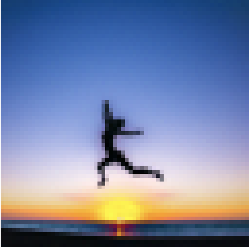
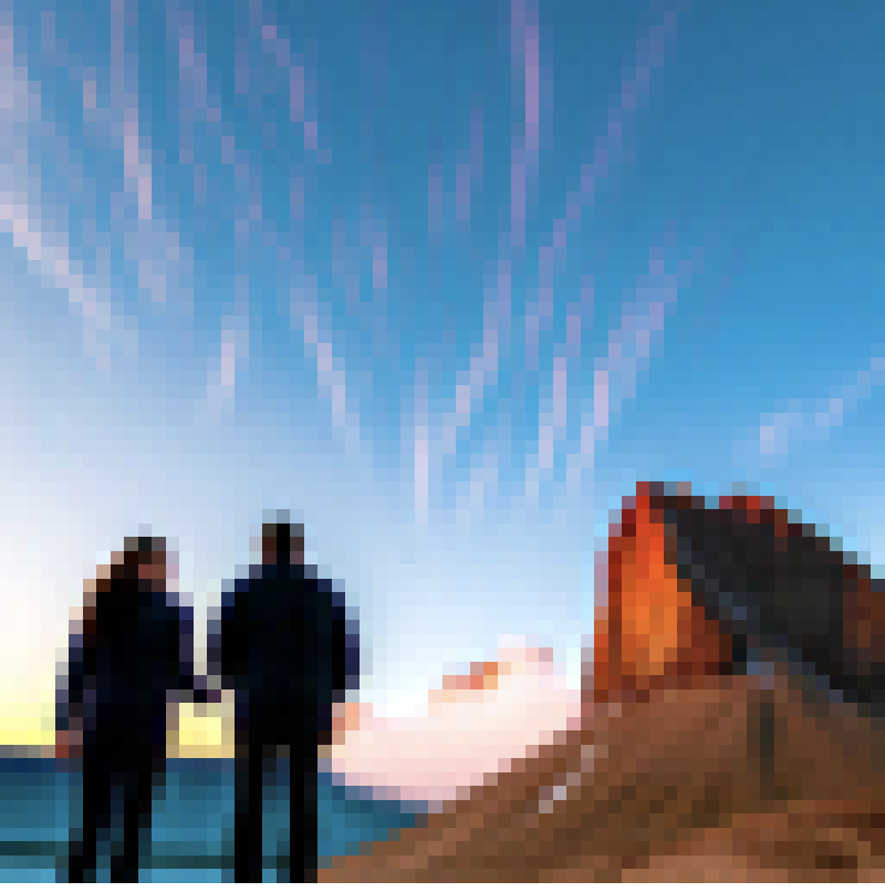
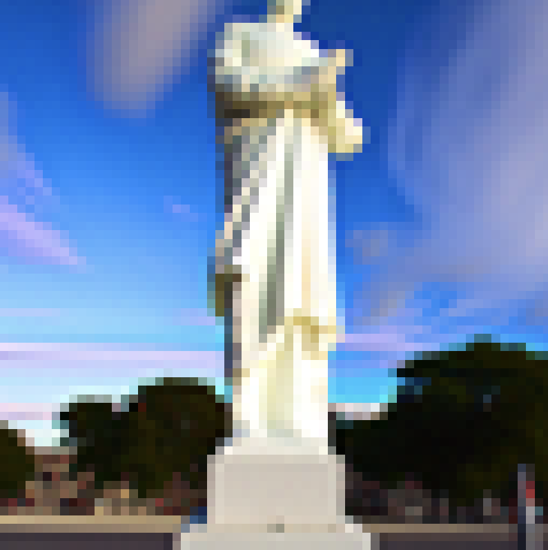
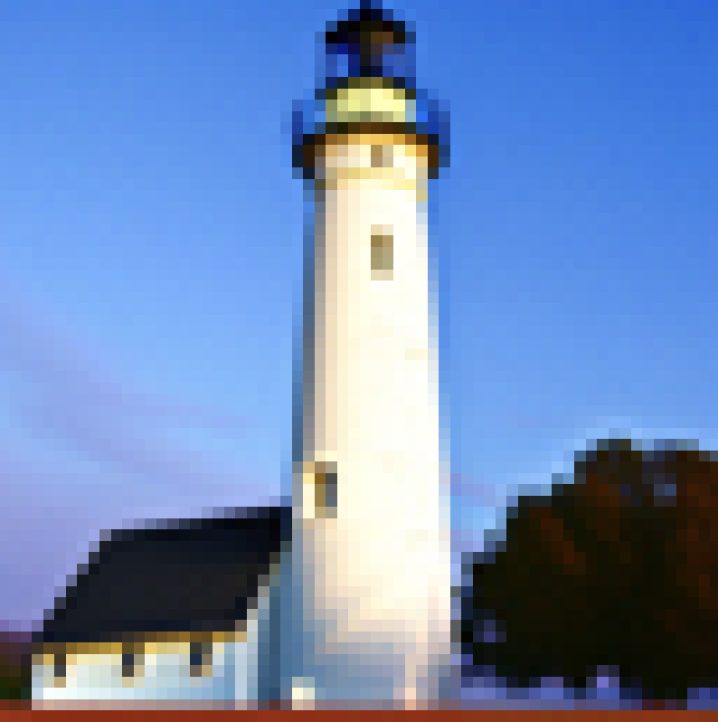
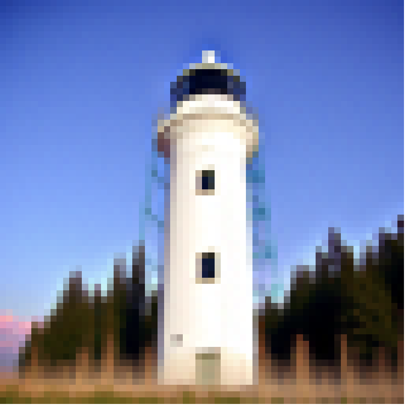
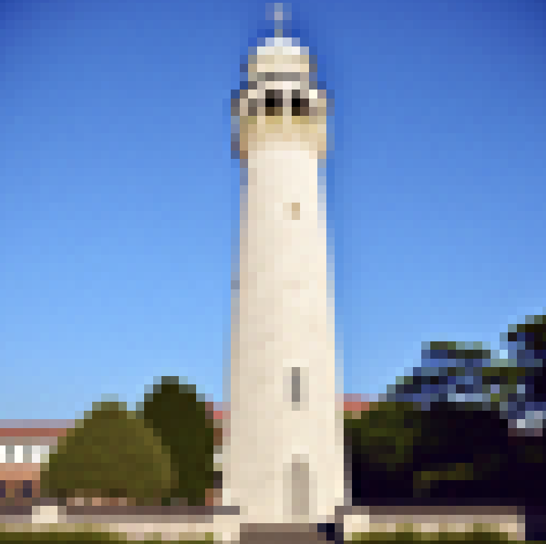
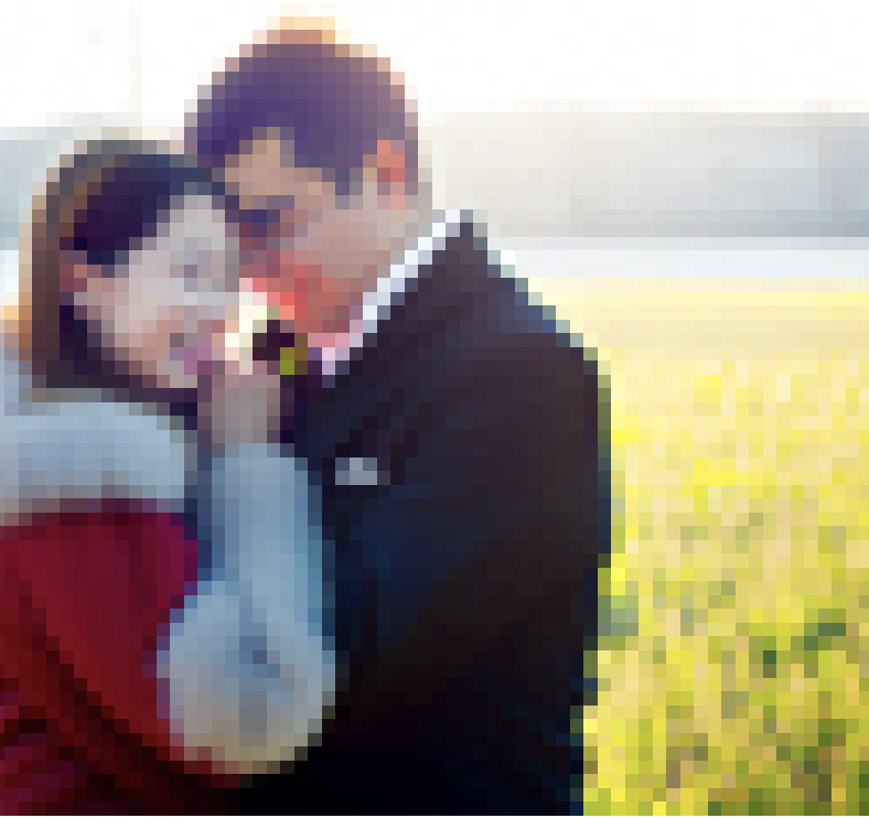
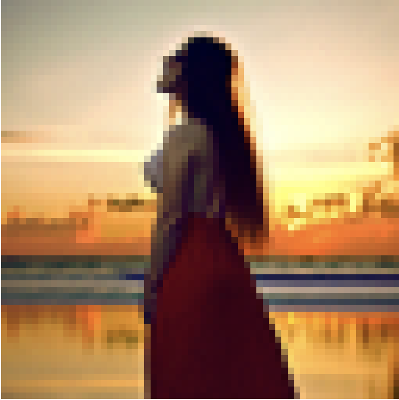
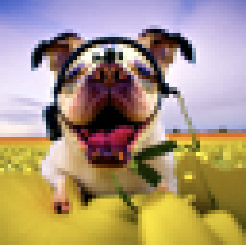
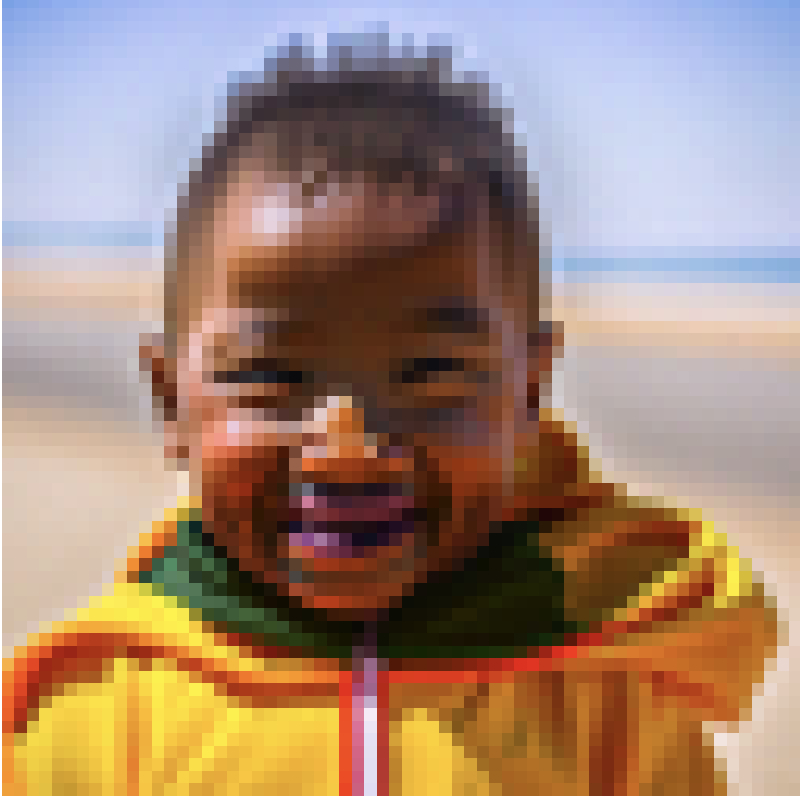
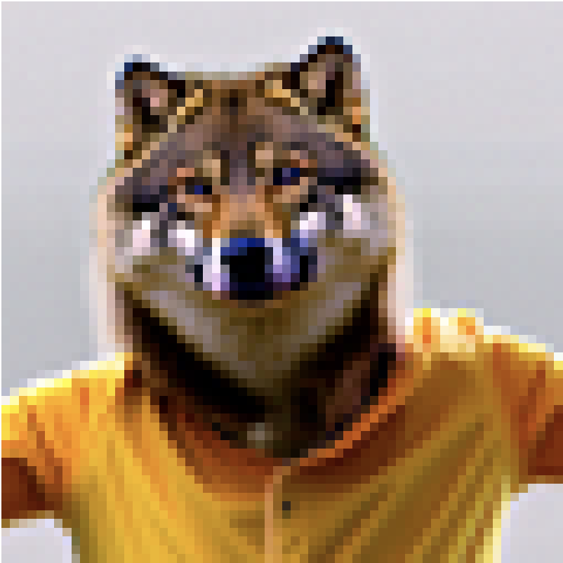
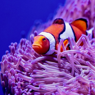
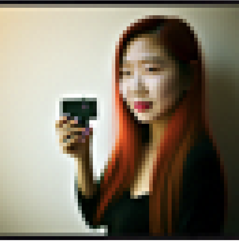
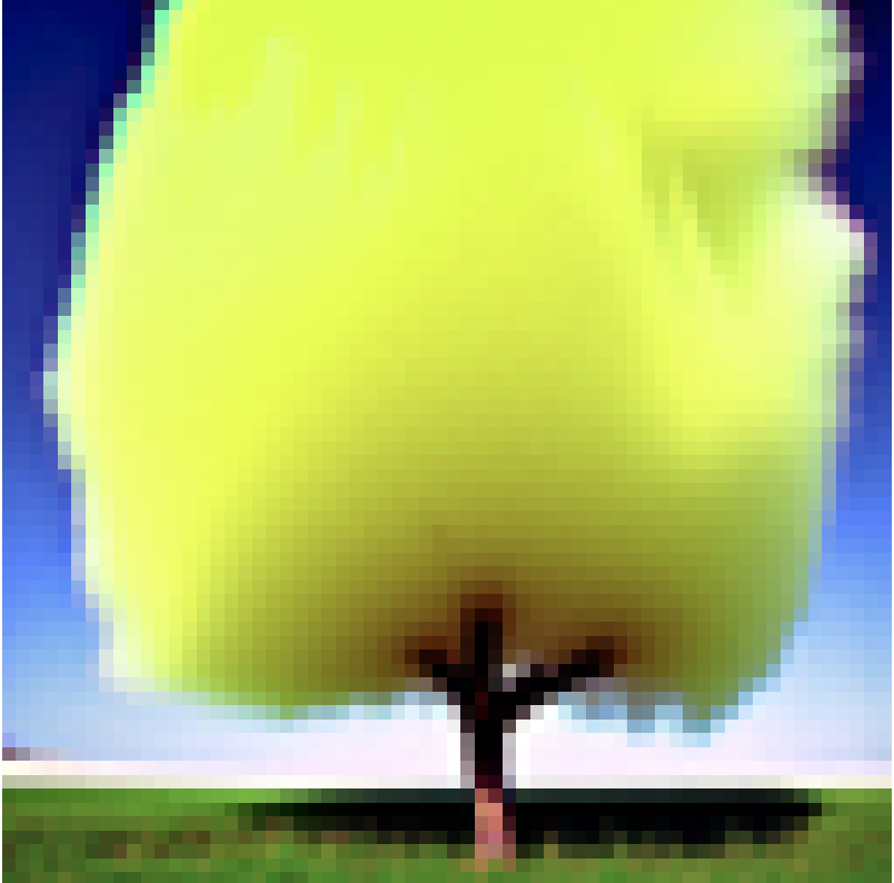
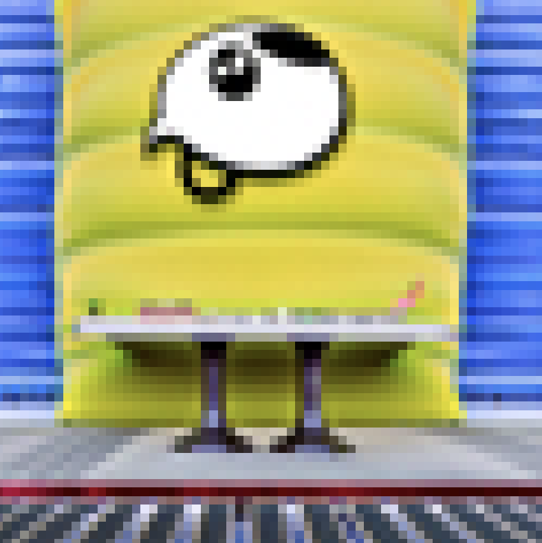
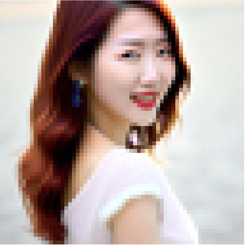
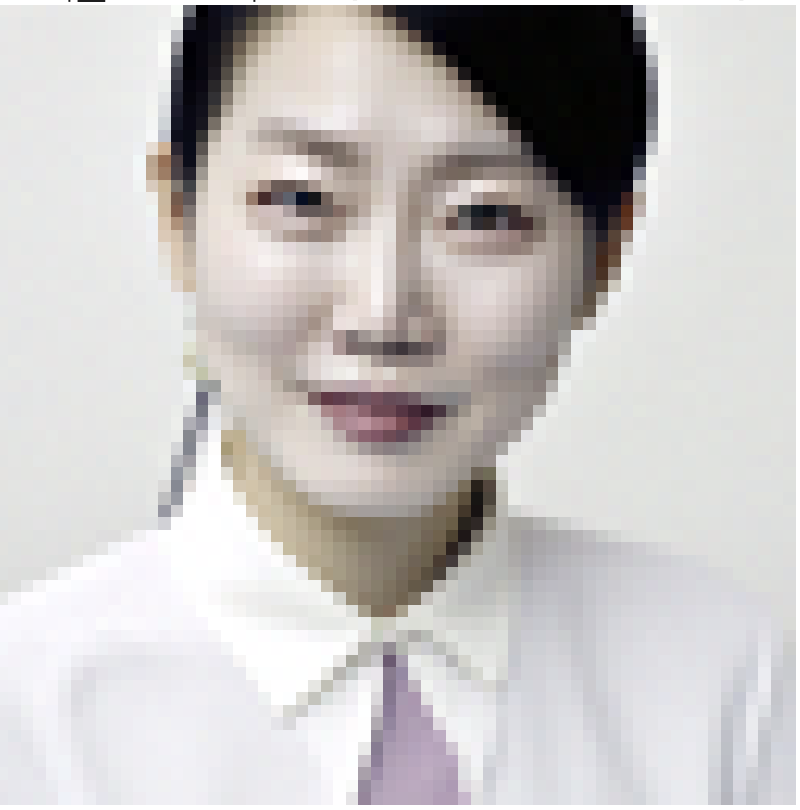
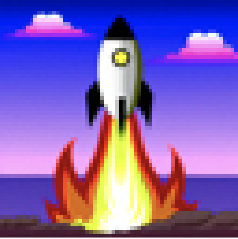
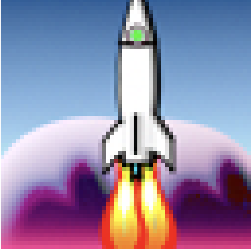
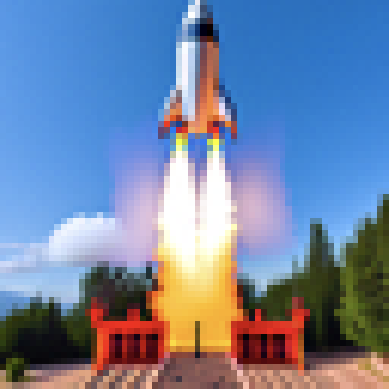
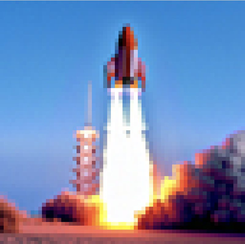
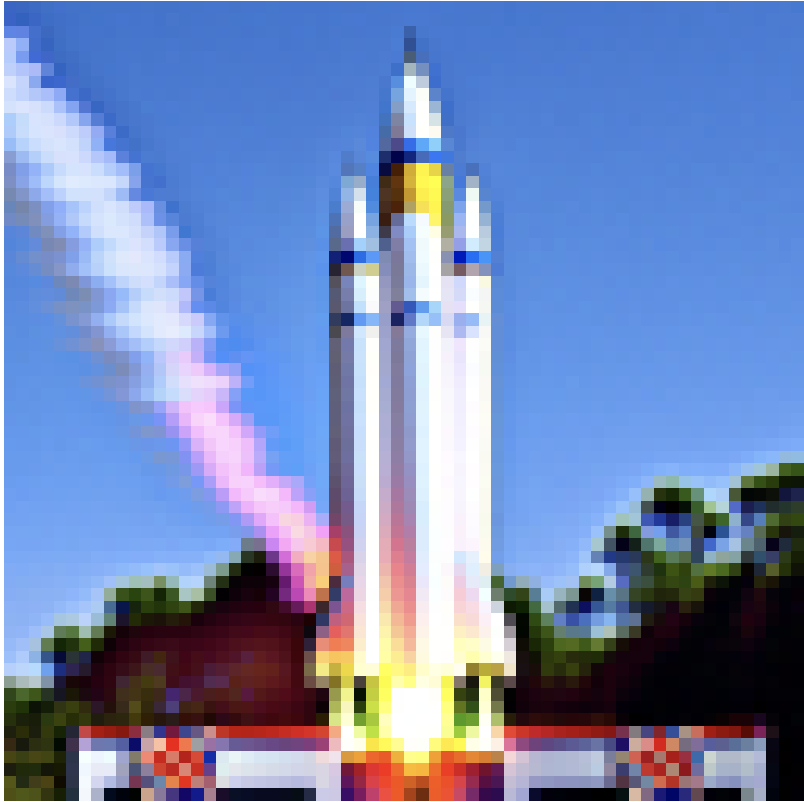
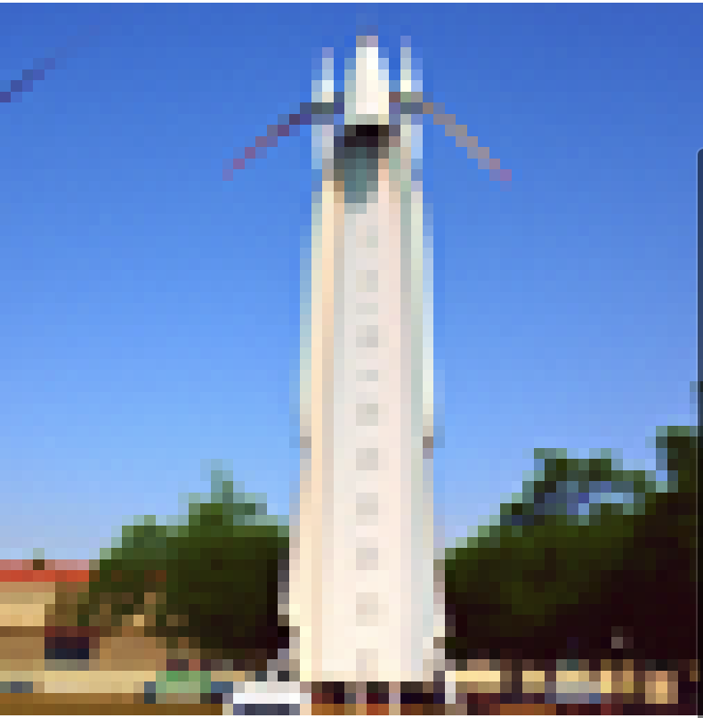
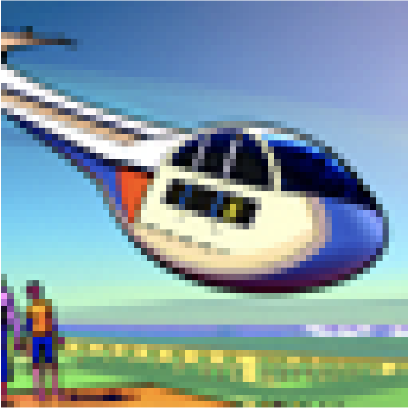
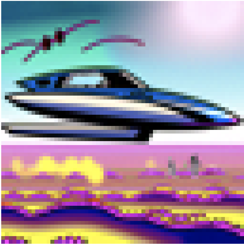
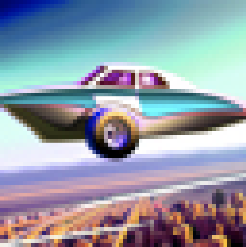
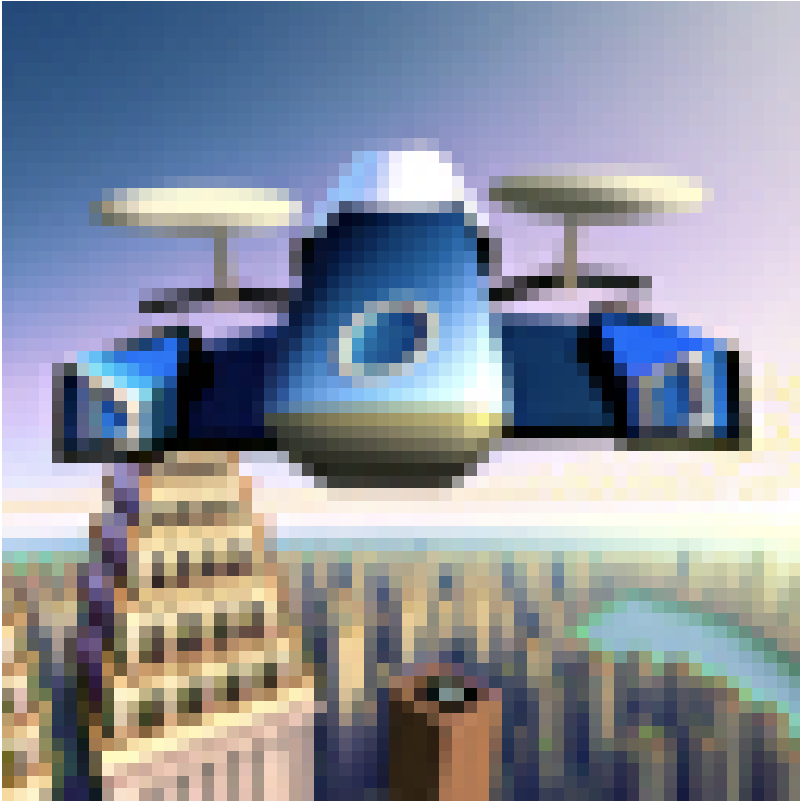
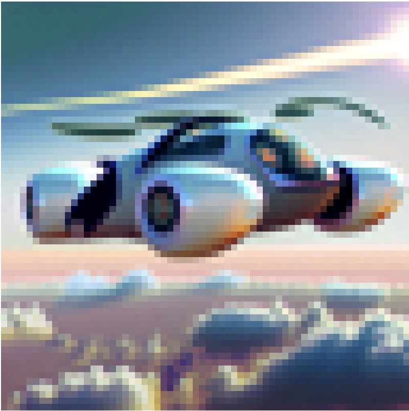
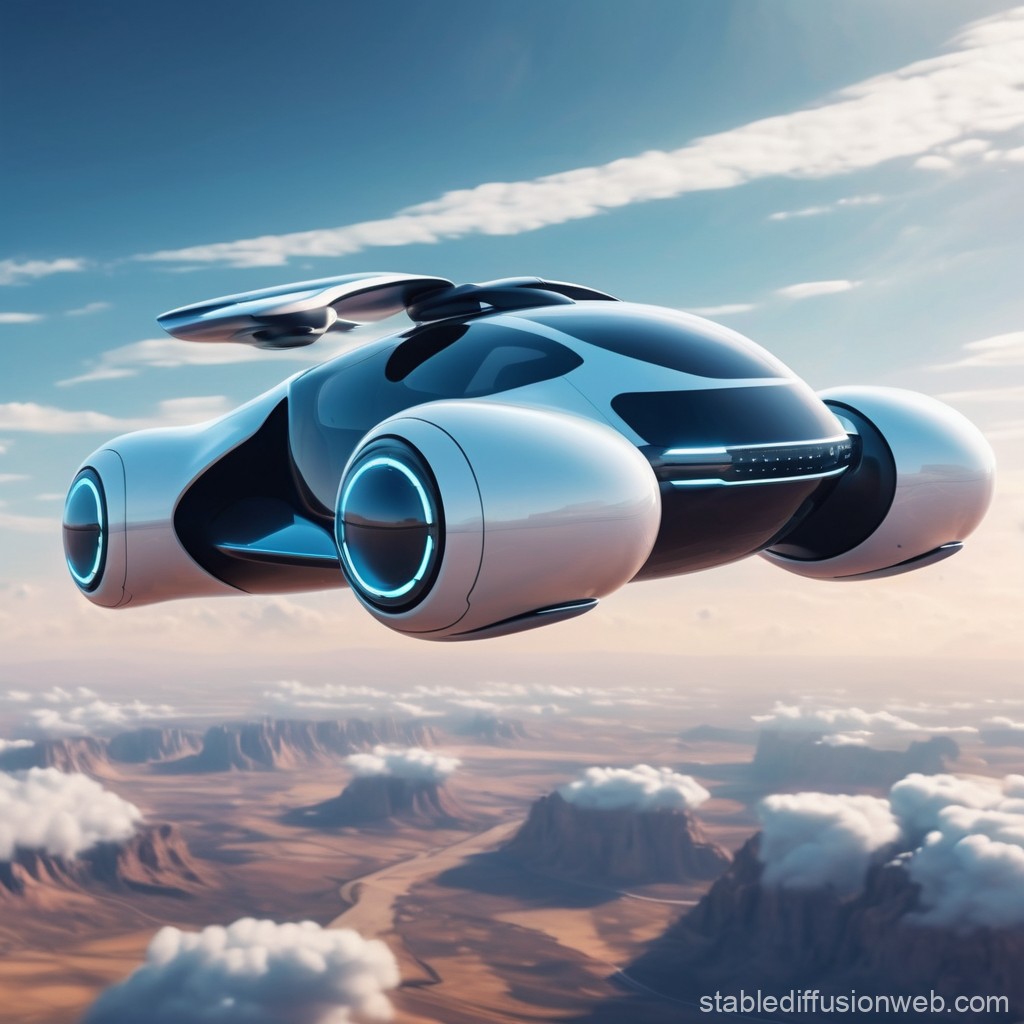
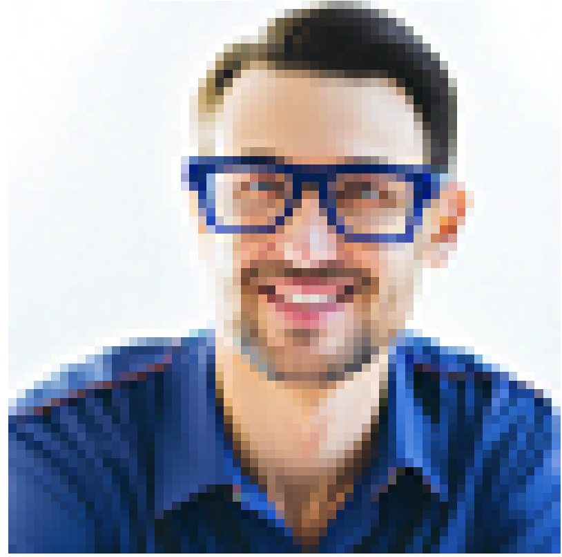
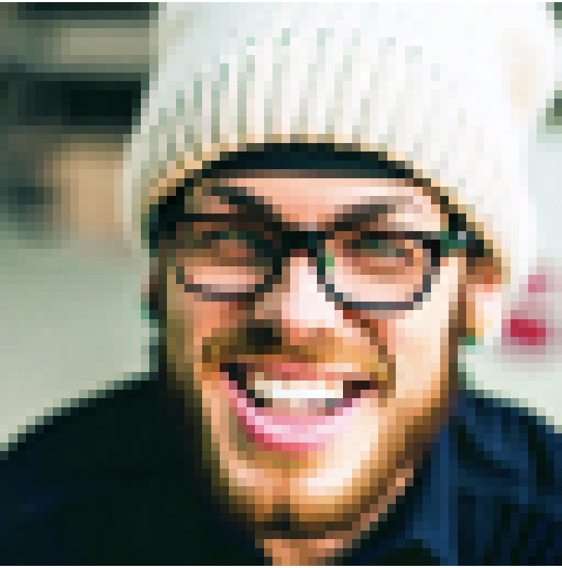
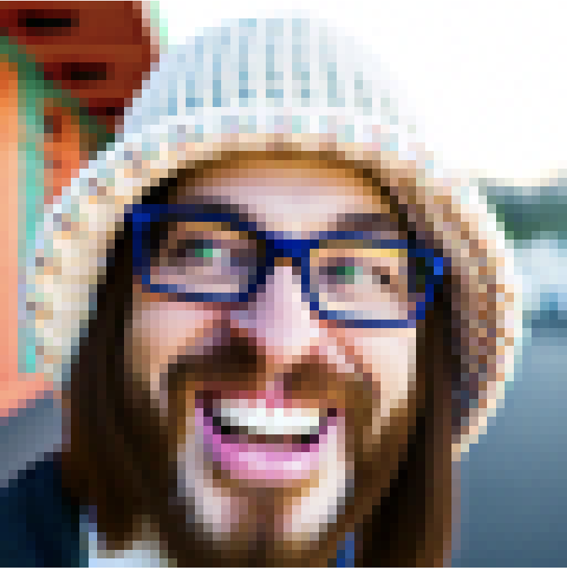
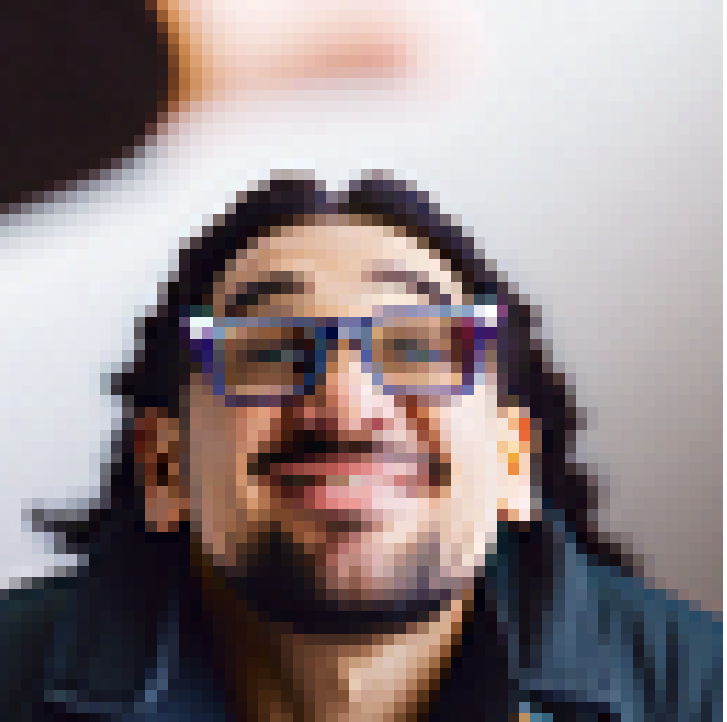
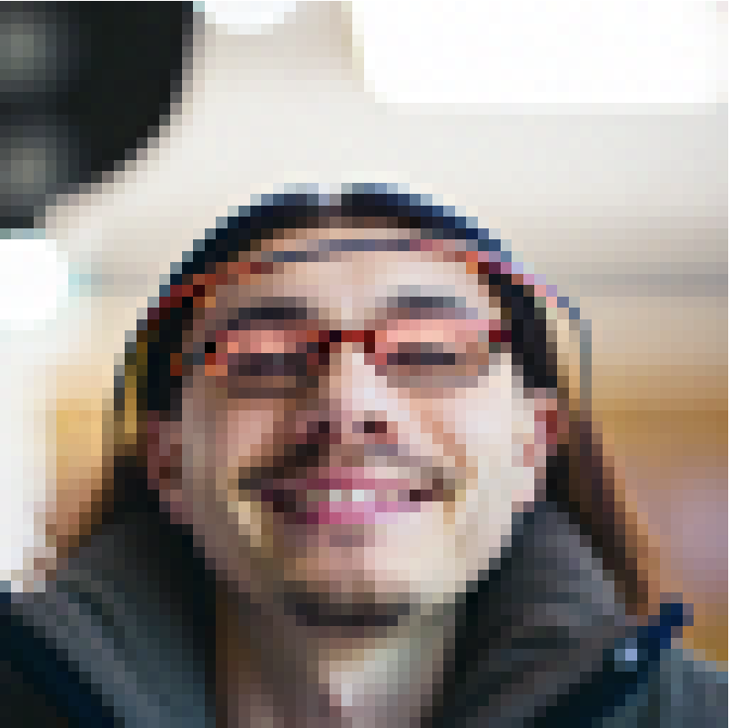
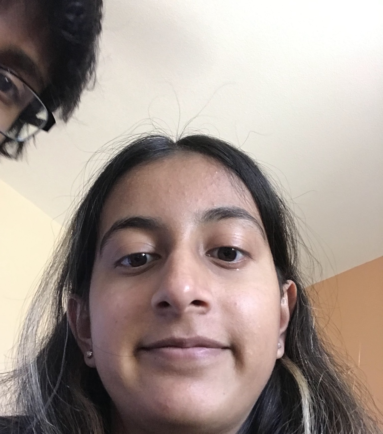
The idea behind this project was to use premade diffusion models for image generation, as well as training my own diffusion model. Some examples of results from this project are shown below.
Implementing the Forward Process
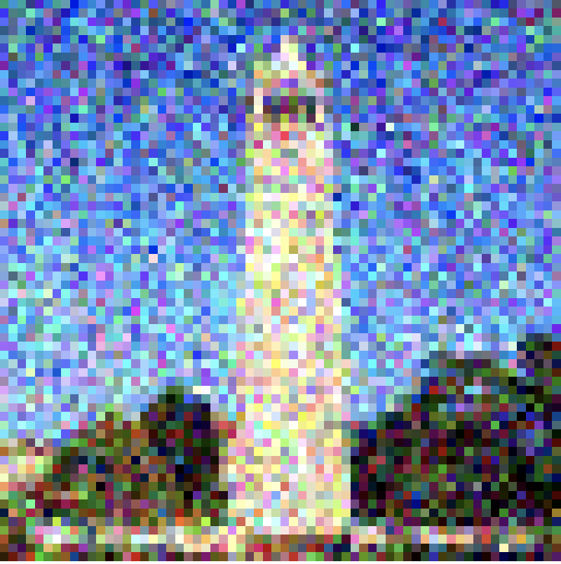
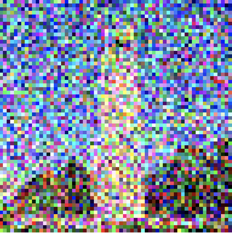
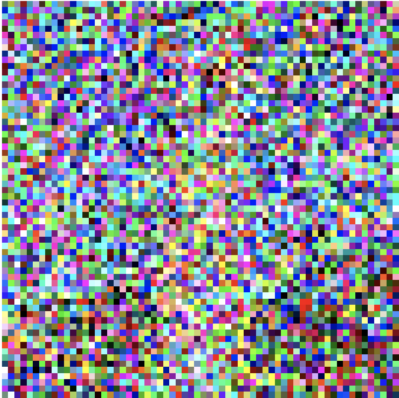
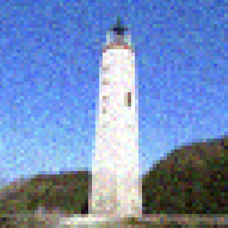
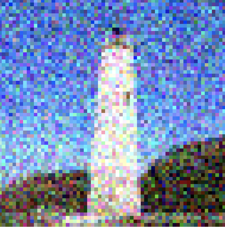
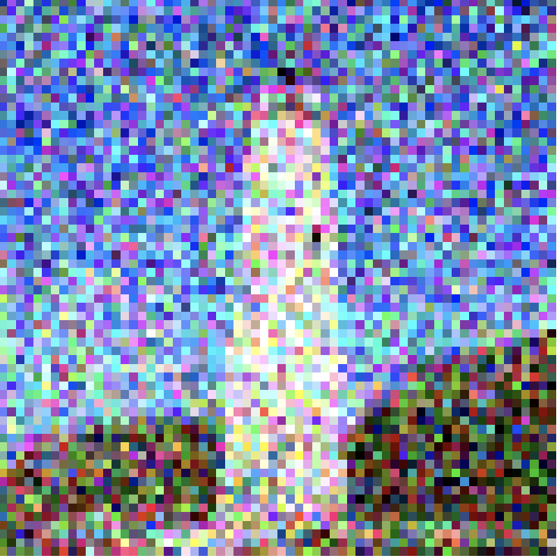
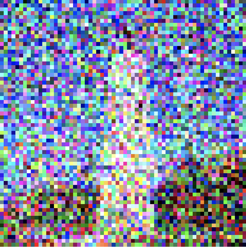
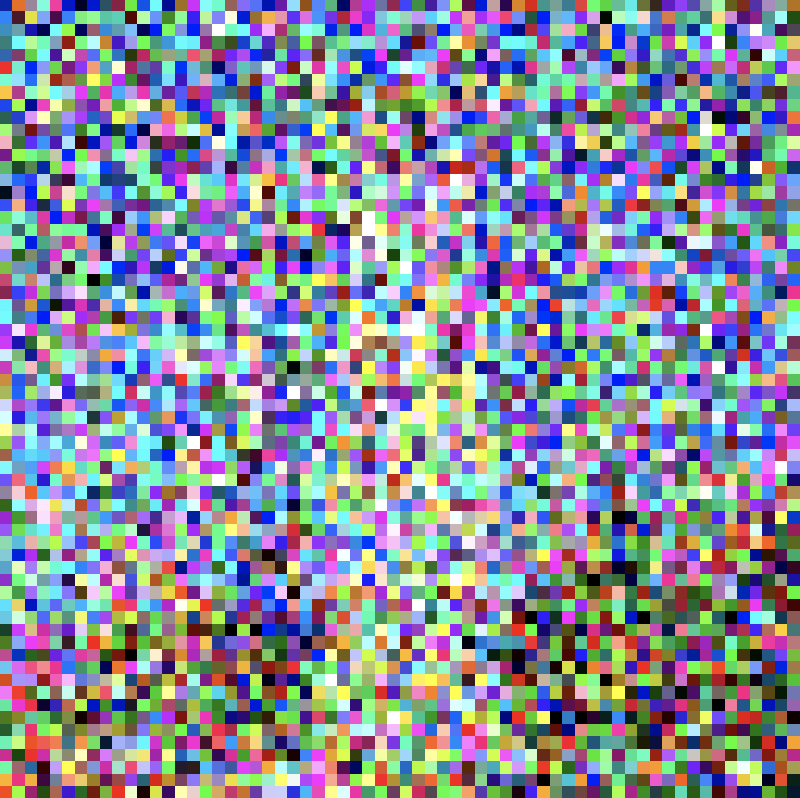
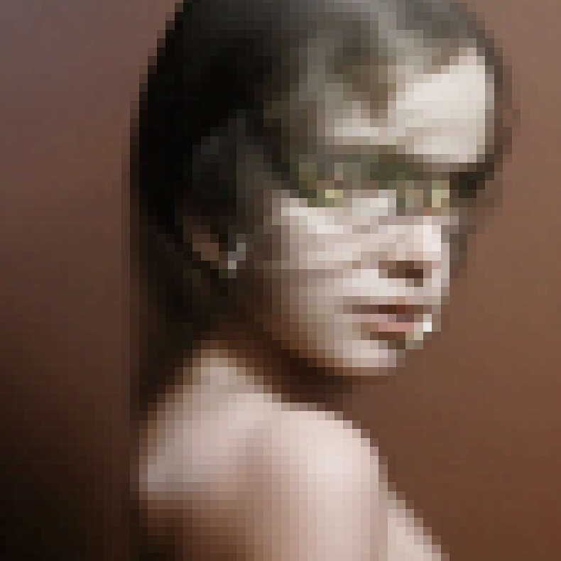
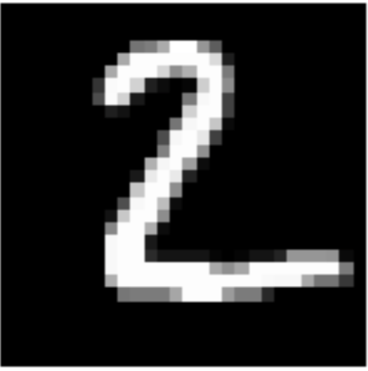
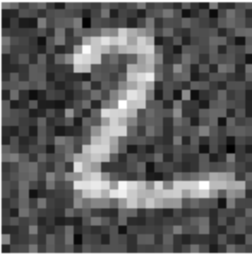
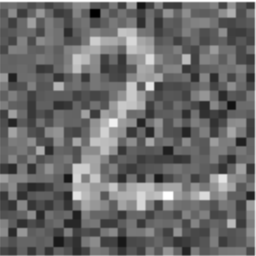
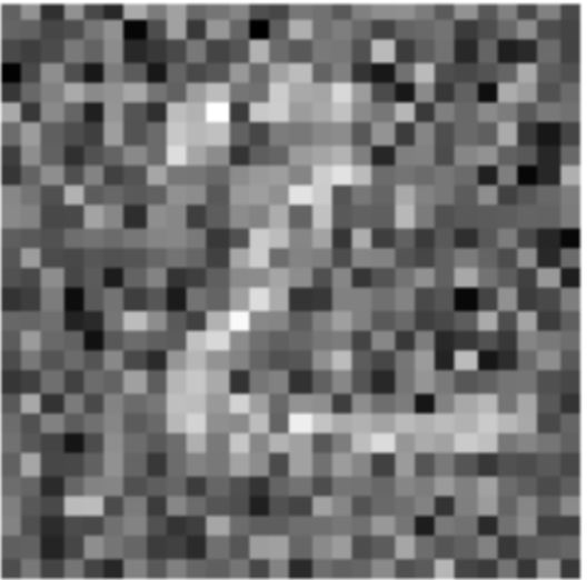
The first step of this project was creating a way to add noise to any image. Taking in an image and a timestep on the range [0, 1000], where 0 represents the clean image and 1000 is pure noise, I used the following equation to output the image with a certain amount of noise.
\[ {x}_t = \sqrt{\bar{\alpha}_t} {x}_0 + \sqrt{1 - \bar{\alpha}_t}\epsilon \quad \text{where} \quad \epsilon \sim \mathcal{N}(0, 1) \] \[ \bar{\alpha_t} \text{ represents the noise coefficient, as chosen by DeepFloyd's creators.} \]
Classical Denoising
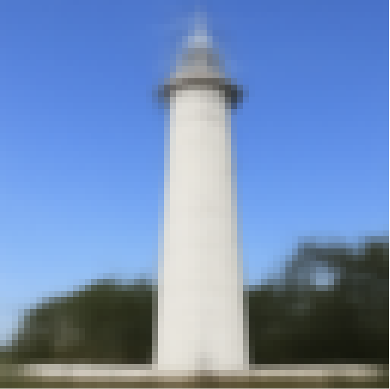
The next step is to take in the noisy images as generated above, and attempt to 'denoise' them. The next couple of sections will investigate different ways to do so.
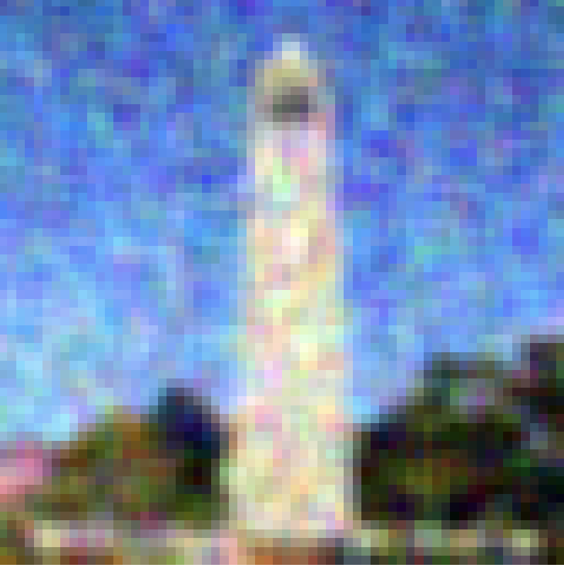
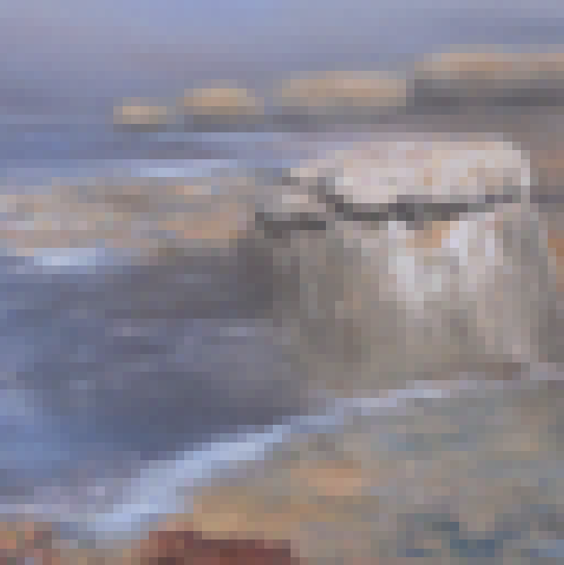
One method in which these images can be noised is simply Gaussian blur filtering. By applying a Gaussian filter, it blurs the image, but it gives poor results, as demonstrated below.
One Step Denoising
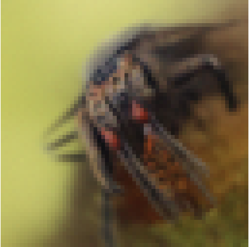
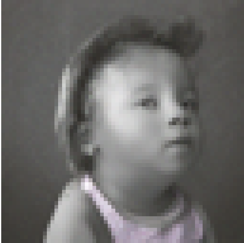
The results of using classical denoising are subpar. We can use the convolutional neural net UNet in order to achieve better results. This model is trained on a vast number of image pairs, between their noisy and denoised forms. This can predict Gaussian noise added to an image, and using this prediction, we can recover an estimate of the original image.
This section demonstrates one step denoising, where we pass in the noisy image as well as its timestep, and the model makes a single prediction about the noise. The examples of the noisy and the one step denoised images are below.
Iterative Denoising
The above one step denoising does provide better results. We can build on this by having the model predict the nois at each timestep, instead of entirely at once. The denoising is iteratively applied at each timestep, from our start to t = 0, which is the denoised image. The output of this is shown below for each of the timesteps, as well as the results of the other methods for comparison.

Sampling from the Diffusion Model
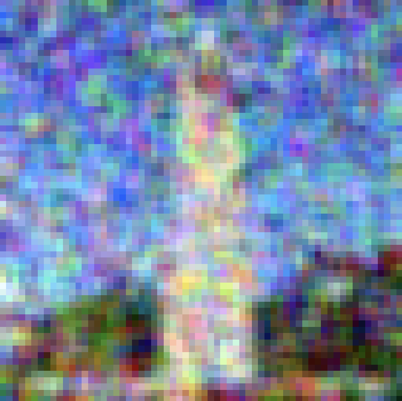
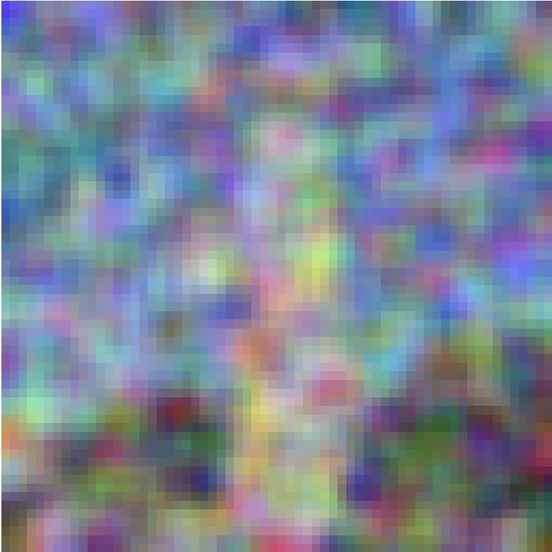
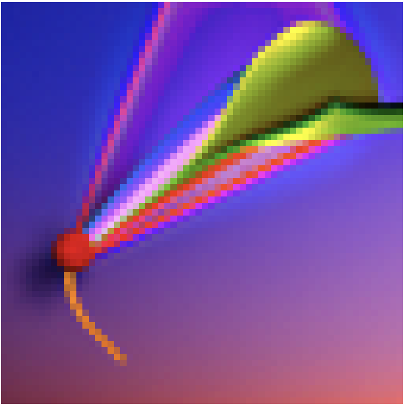
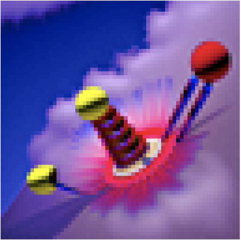
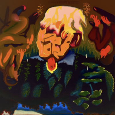
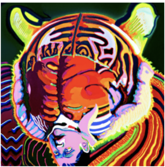
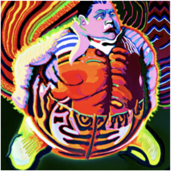
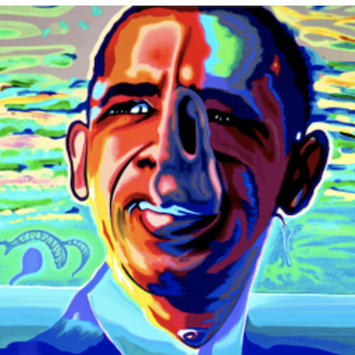
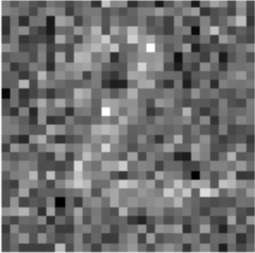
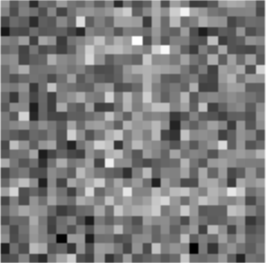
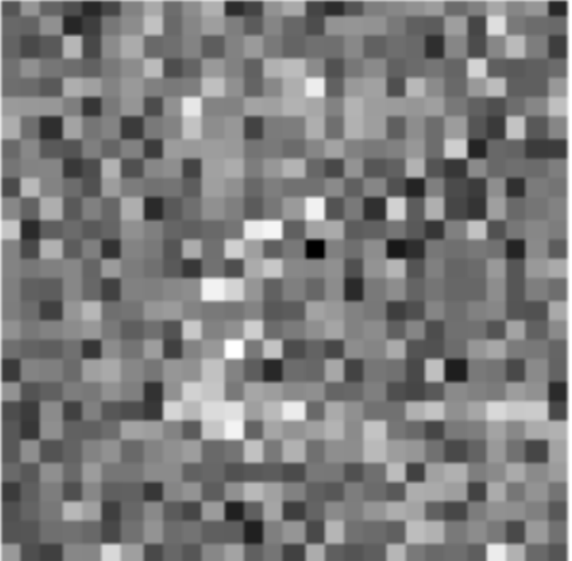
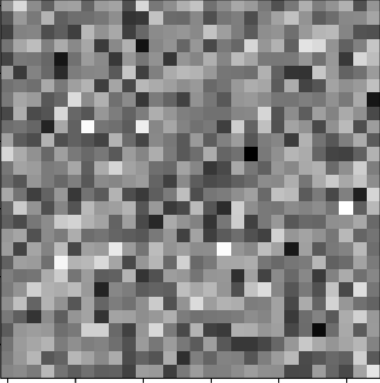
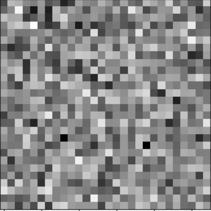
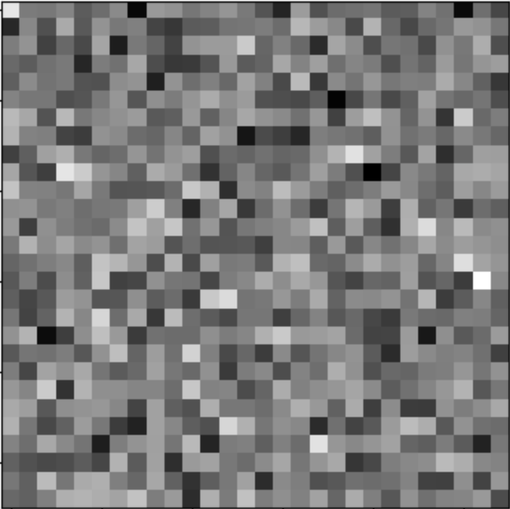
We used the model above to predict noise based off an image that we already had, from a set timestep. However, we can generalize this to simply set out timestep to to the maximum, and pass in an image of complete noise. This essentially samples random images from the UNet model. 5 examples of this are shown below.
Classifier-Free Guidance
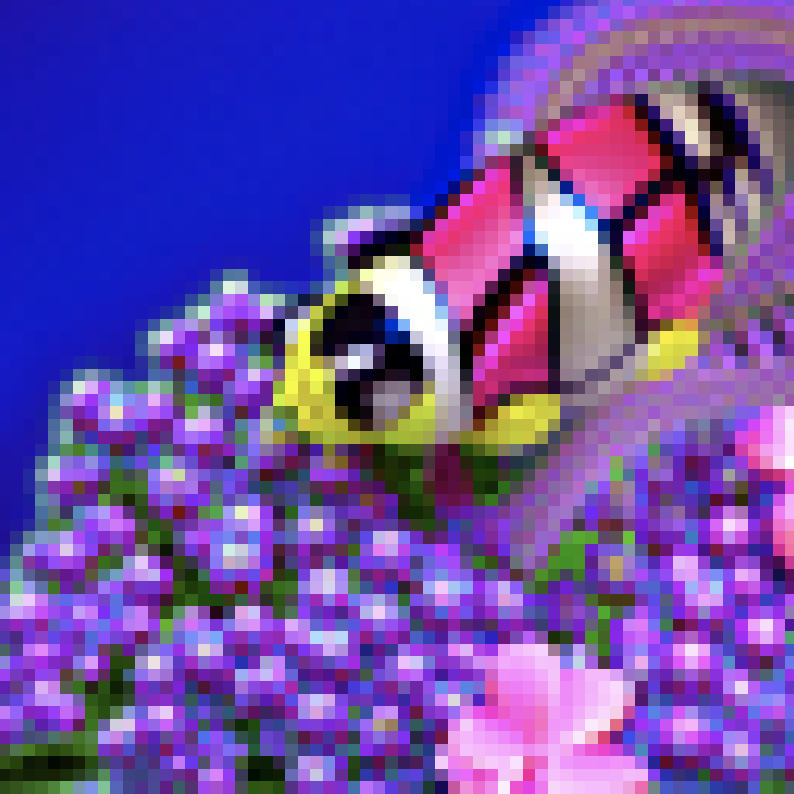
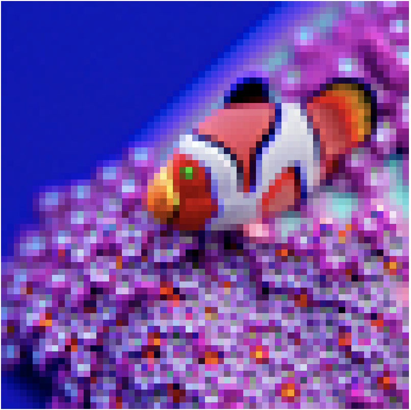
The images generated above are unique, but not very realistic. One way we can generate better images is through classifier-free guidance. We can update our noise prediction to use a combination of unconditional and conditional noise, as demonstrated in the equation below. This yields improved results than before.
\[ \epsilon = \epsilon_u + \gamma(\epsilon_c - \epsilon_u) \quad \] \[ \text{where} \quad \gamma \quad \text{is the strength of the CFG} \]
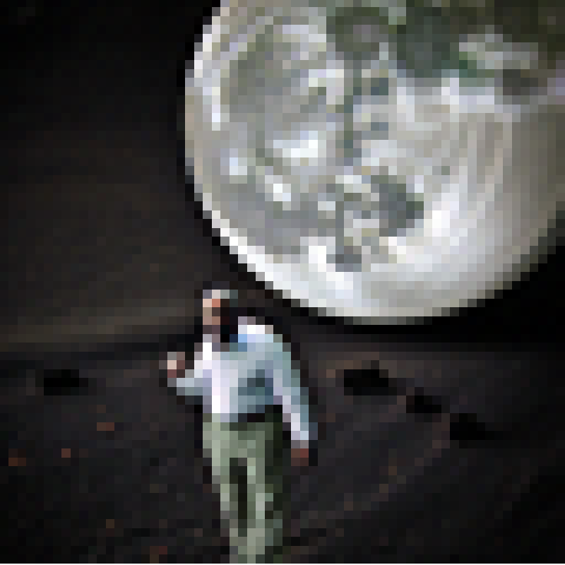
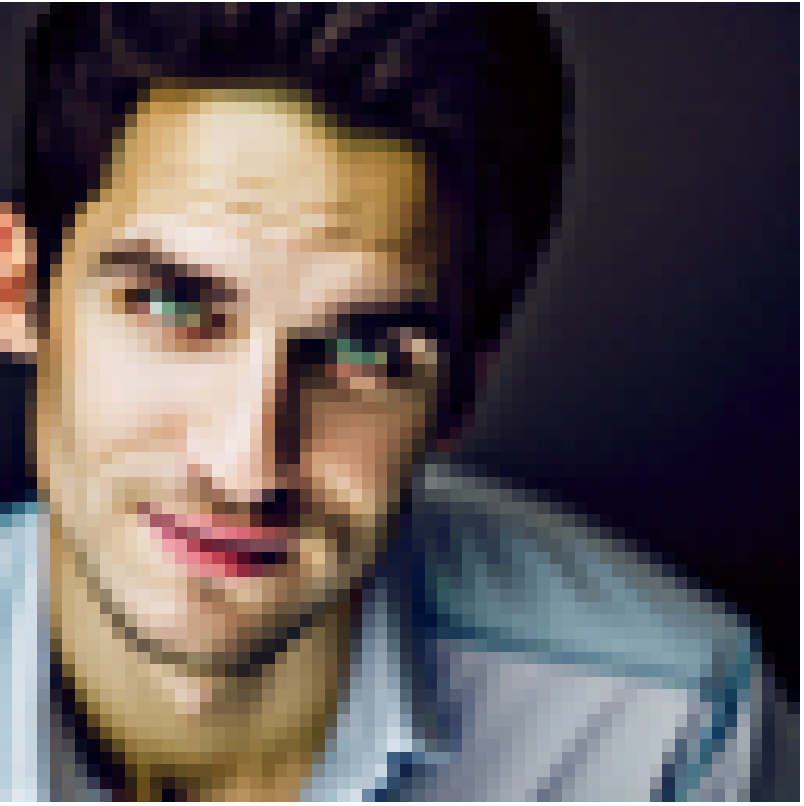
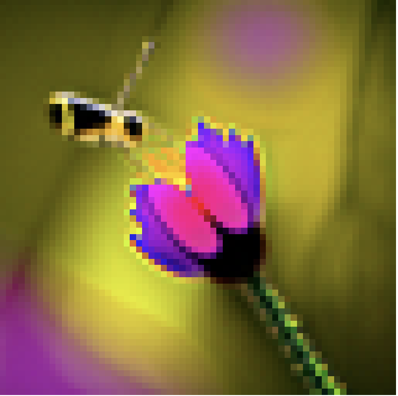
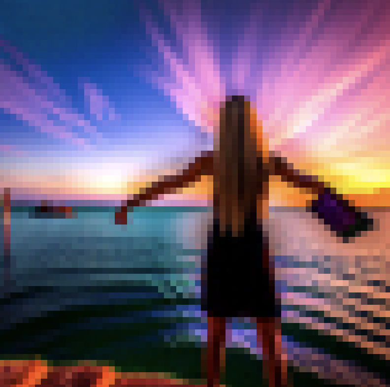
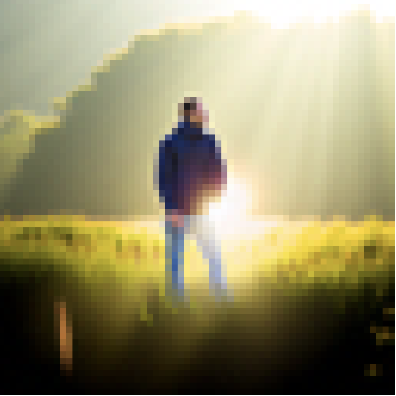
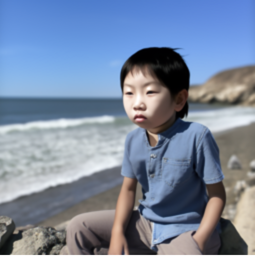
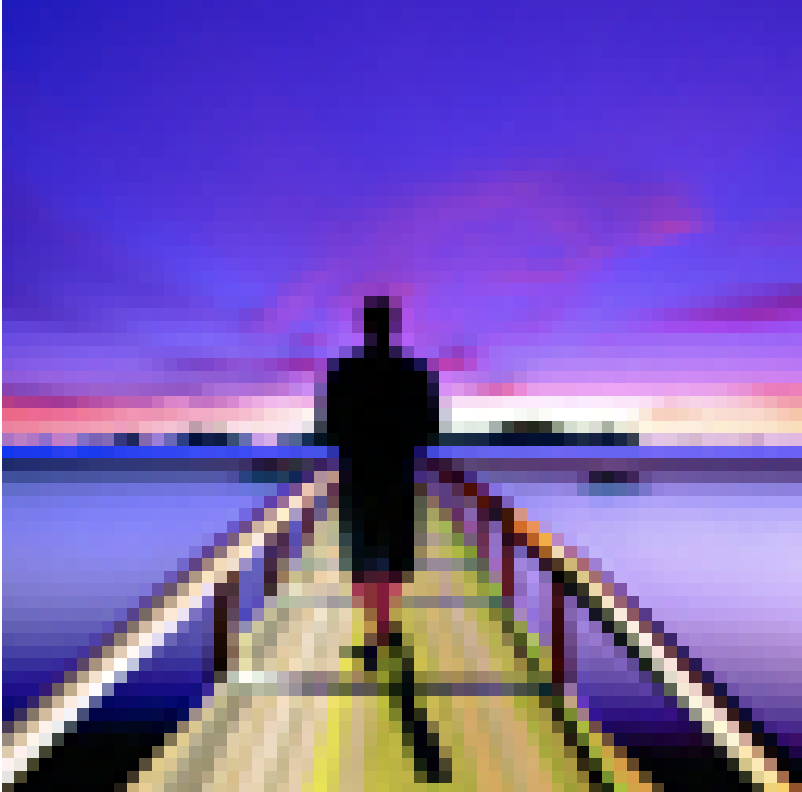
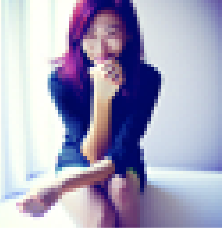
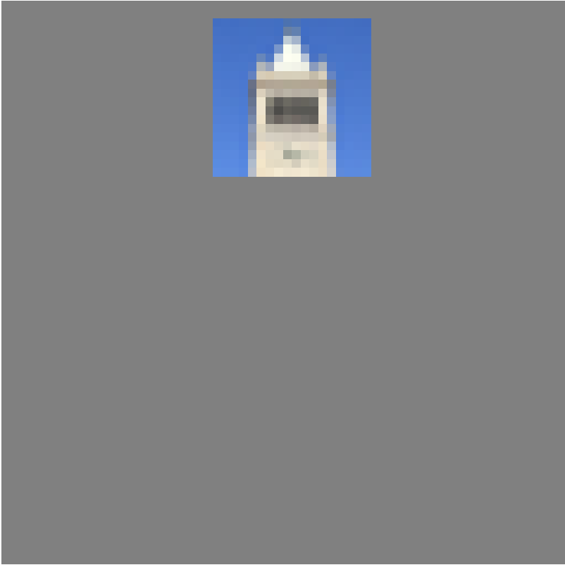
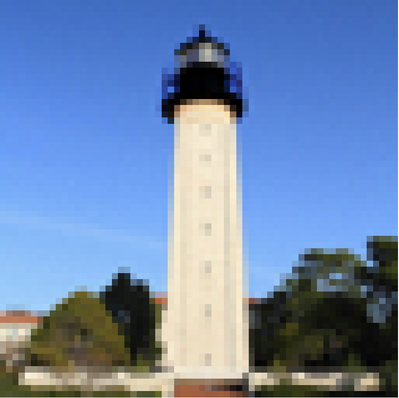
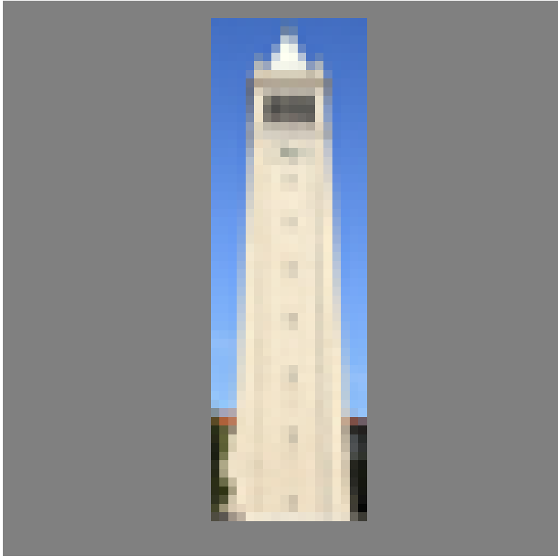
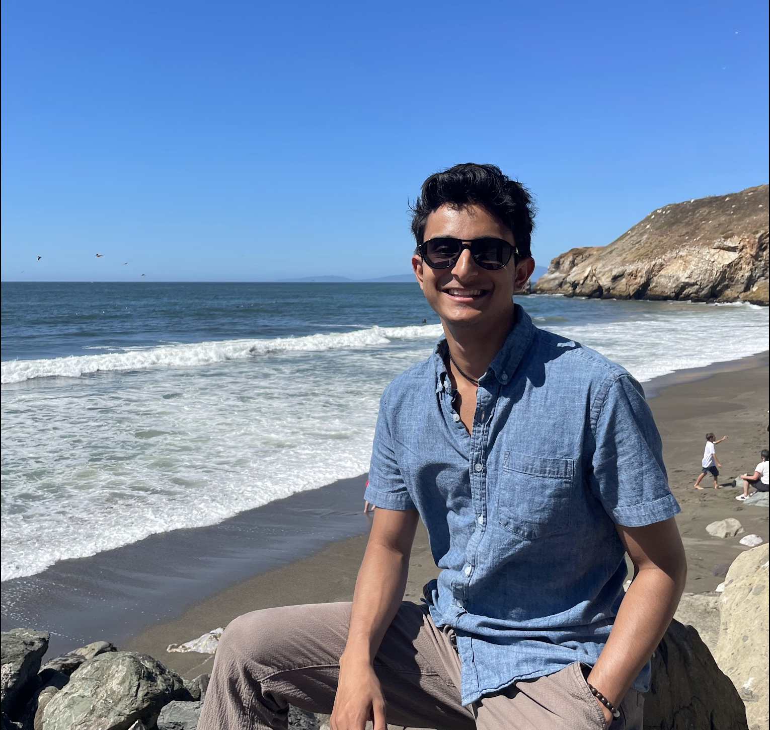
Image to Image Translation
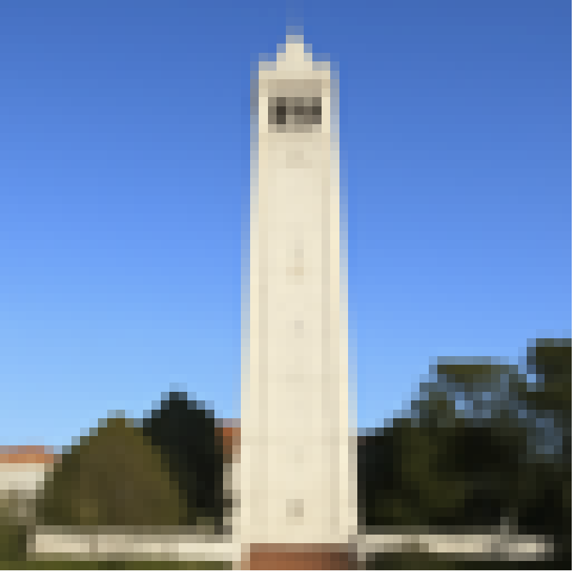
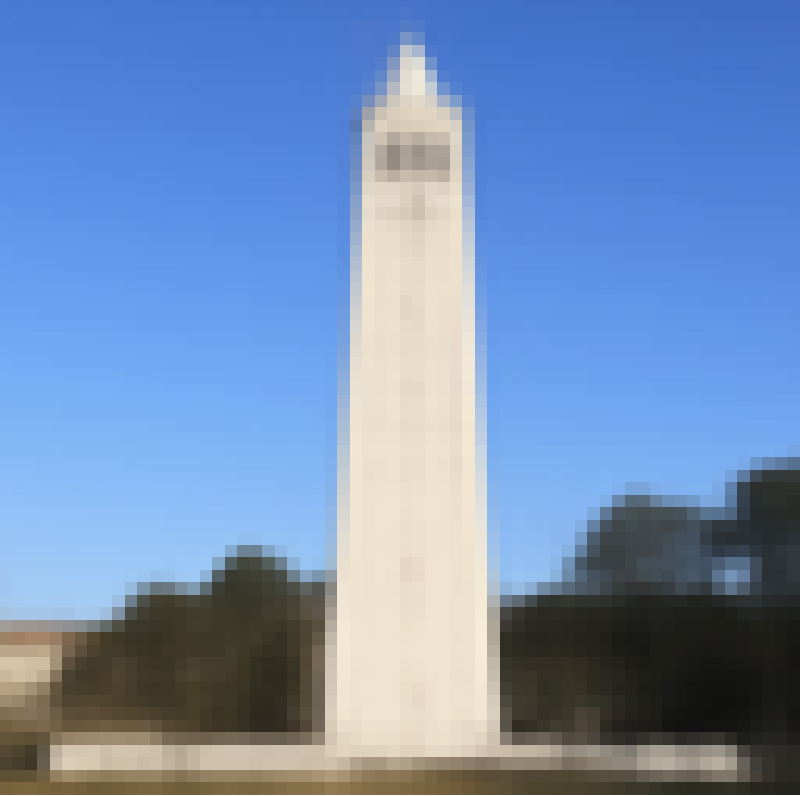
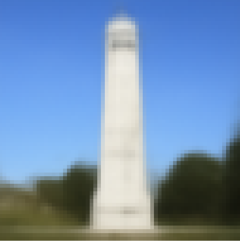
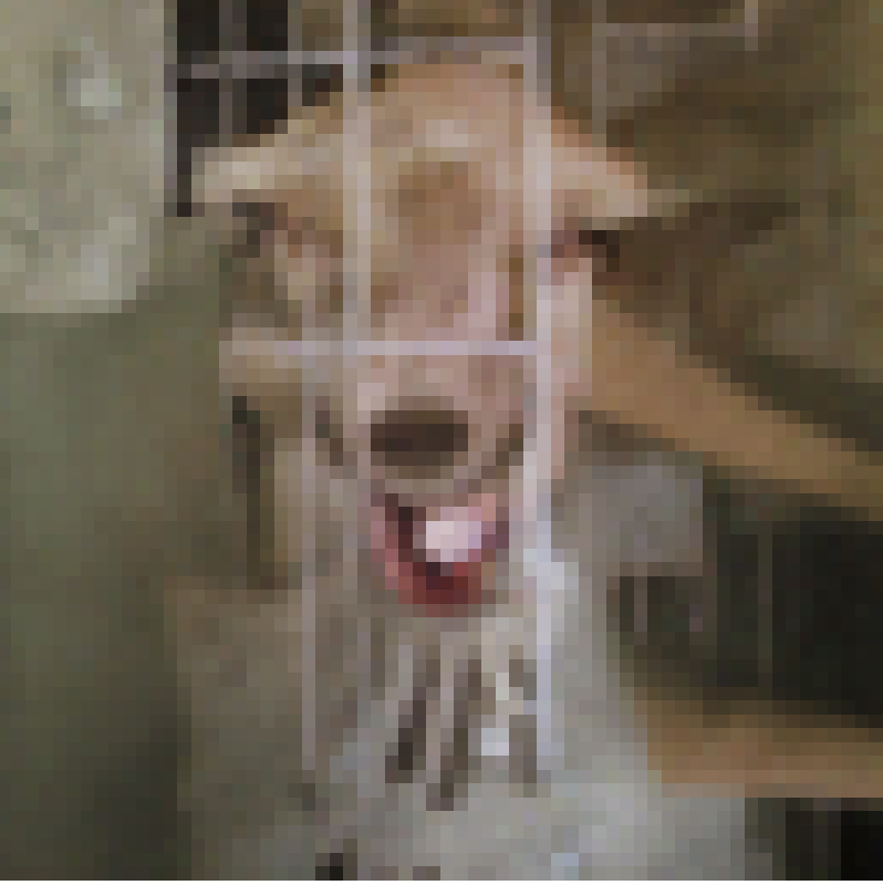
A similar process can be followed for producing image translations. By blurring the image at different levels, and then trying to predict the original image, we can create a range of pictures, with each one getting more and more similar to the original image. The i_start variable represents where we start our image from, with lower values meaning higher noise is added at the beginning, and higher values meaning less noise is added.
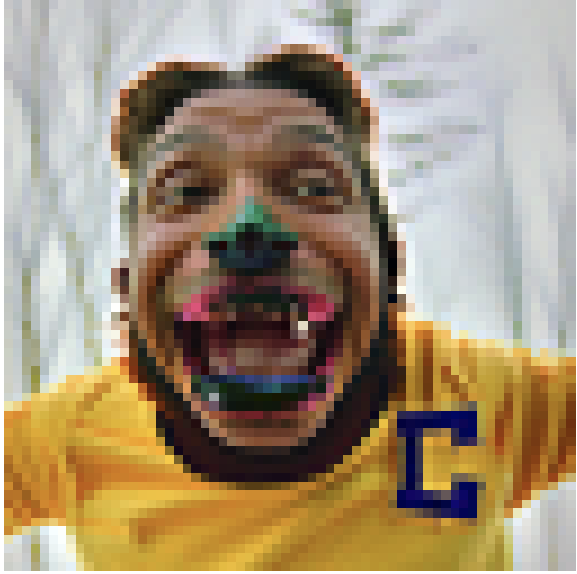
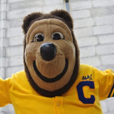
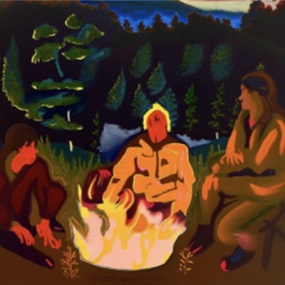
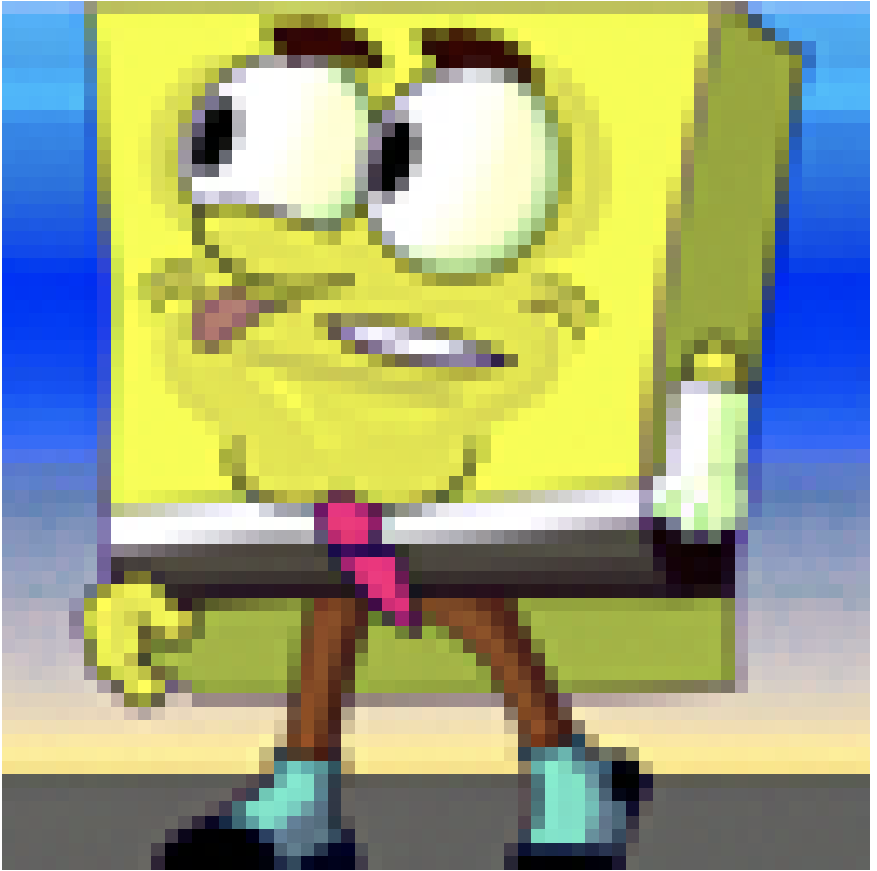
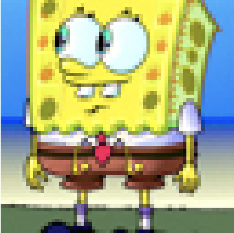
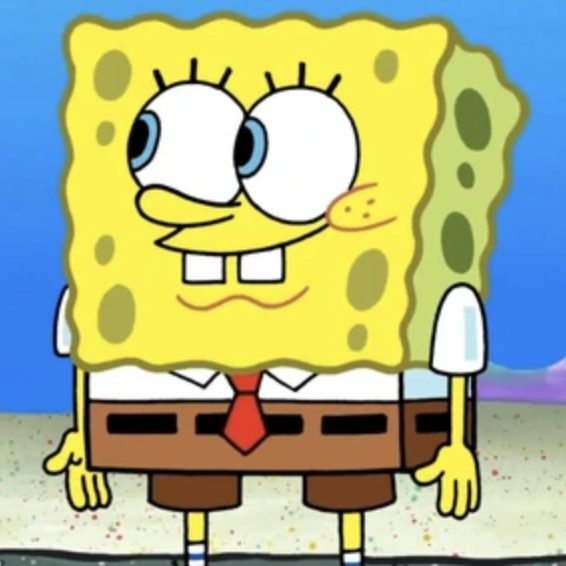
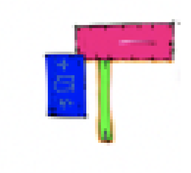
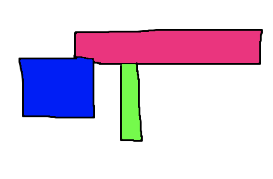
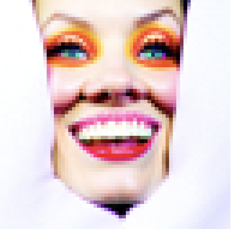
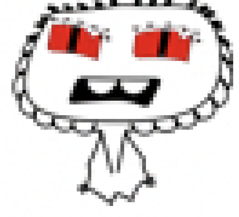
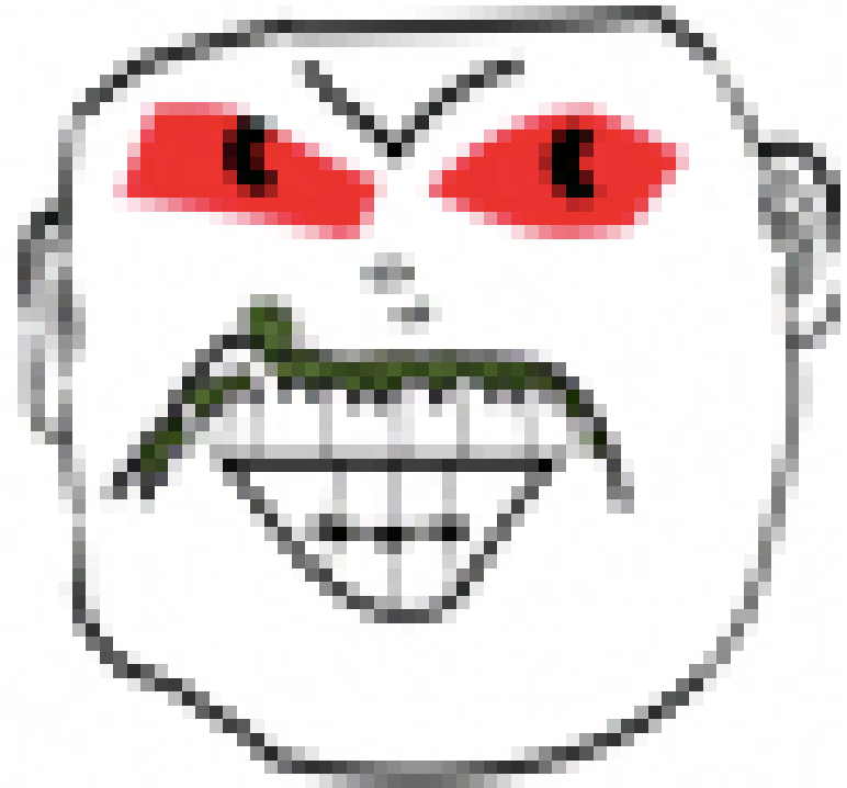
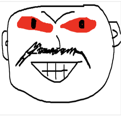
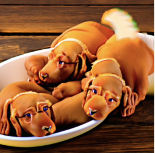
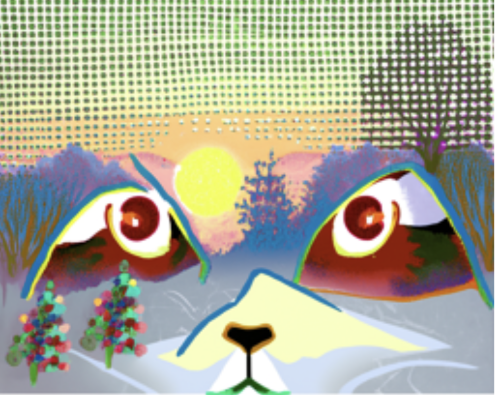
Editing Hand-Drawn Images
This method is particularily interesting with hand drawn images, it can turn anything you draw into something more realistic. I chose one cartoon, as well as two random doodles I made and ran them through this process, and the results are shown below.


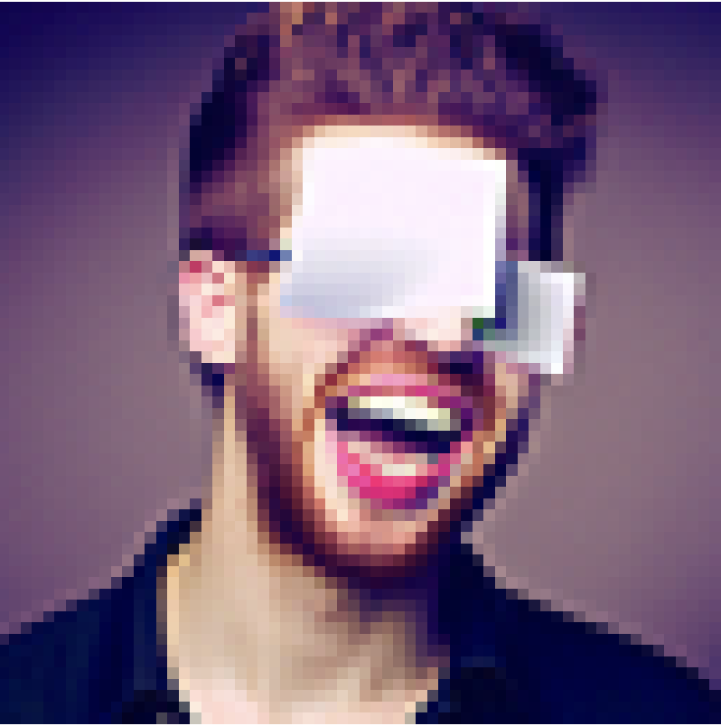
Inpainting
We can follow a similar method in order to accomplish inpainting. This essentially takes in an image and a mask, and predicts only the part inside the mask, while leaving the rest unchanged. At each step, we force the black part of the mask to have the pixels from the original image (with the correct noise added), and the model's output for the mask area is kept. The results of images and their corresponding masks are shown below.


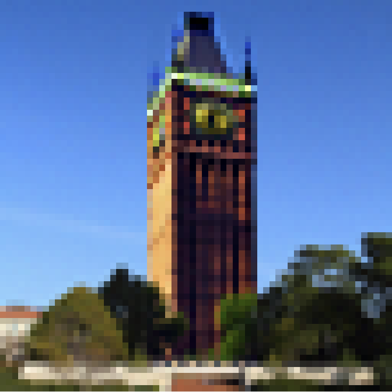
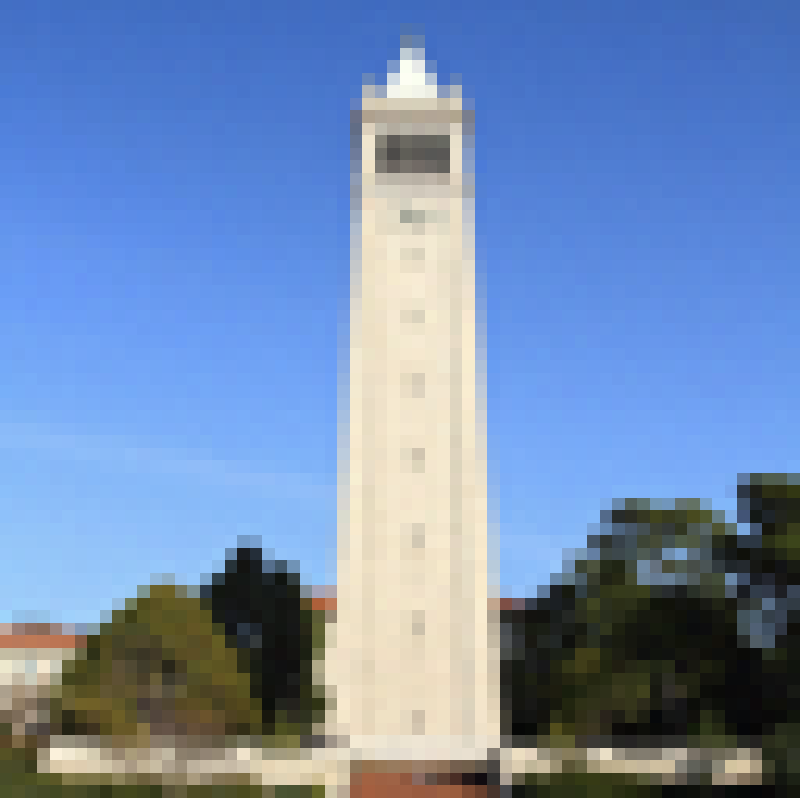
Text Conditional Image to Image Translation
Currently, the model is predicting noise based off of the prompt "a high quality image". If we change the prompt to be something more specific, we can generate images that are closer to that prompt as the noise gets higher. Some examples of this are shown below, with the original image on the right, and the prompt that was given is on the left (where i_start = 1).


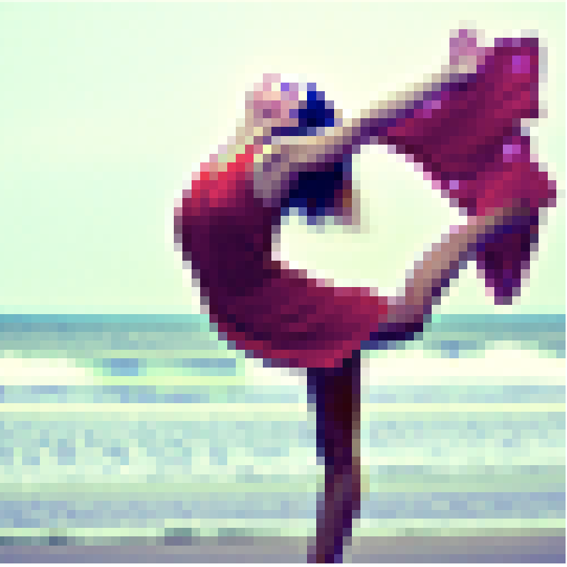
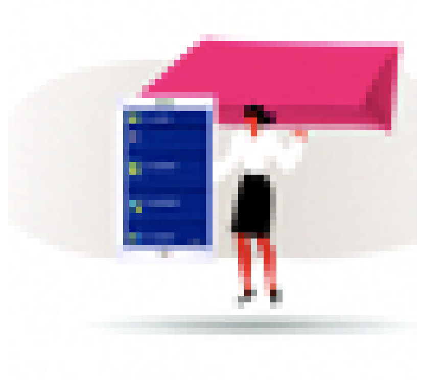
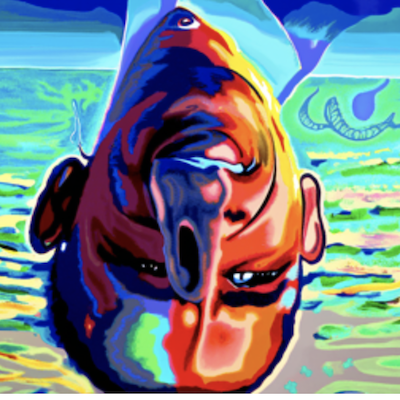
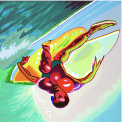
Visual Anagrams
Another unique application of this process is creating a visual anagram. This is where the image appears to be two different things depending on which way it is flipped. To create this, we average the predicted noise of the first prompt, along with the second prompt's predicted noise flipped vertically. The results of this are shown below, you can hover over the image to flip them as well.

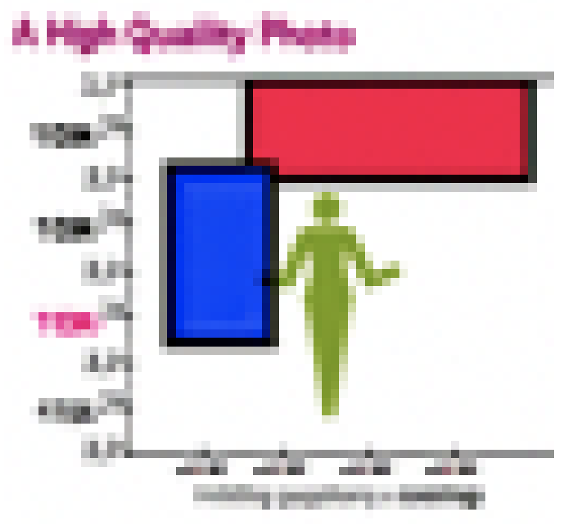
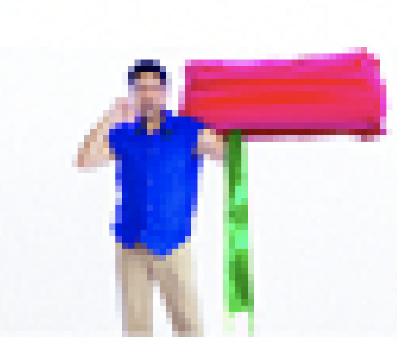
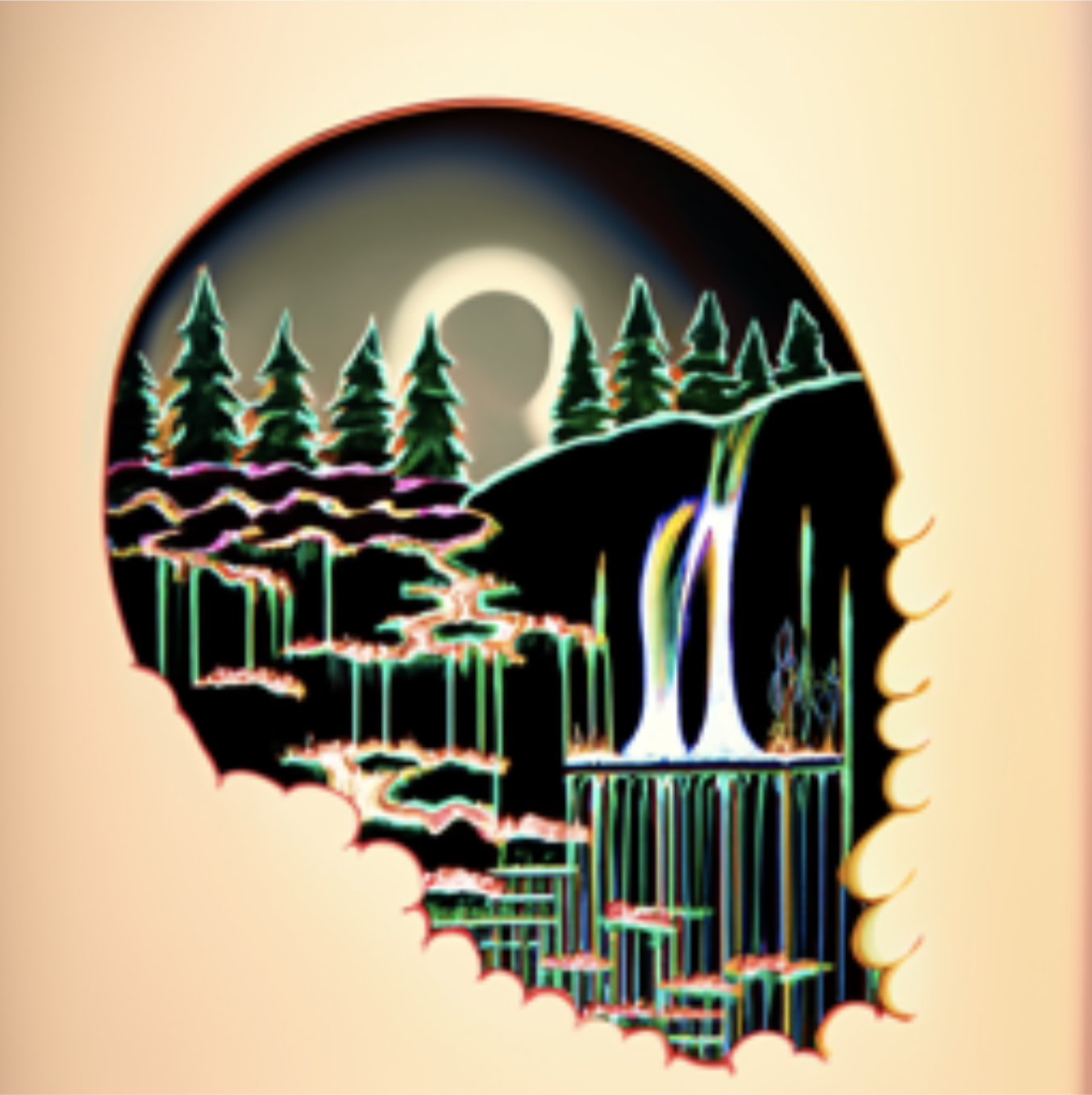
Hybrid Images
Hybrid images are where the image appears to be one thing when up close, but another from afar. In this case, we can predict the noise for two different prompts, and at each step, run one through a high-pass filter, and one through a low-pass filter. This enables us to create the illusions as seen below. Hover over the images to view them zoomed out.
Training a Single-Step UNet
The above sections all rely on a pretrained UNet in order to perform the tasks. The following sections will now investigate how I can train my own model to achieve similar results.
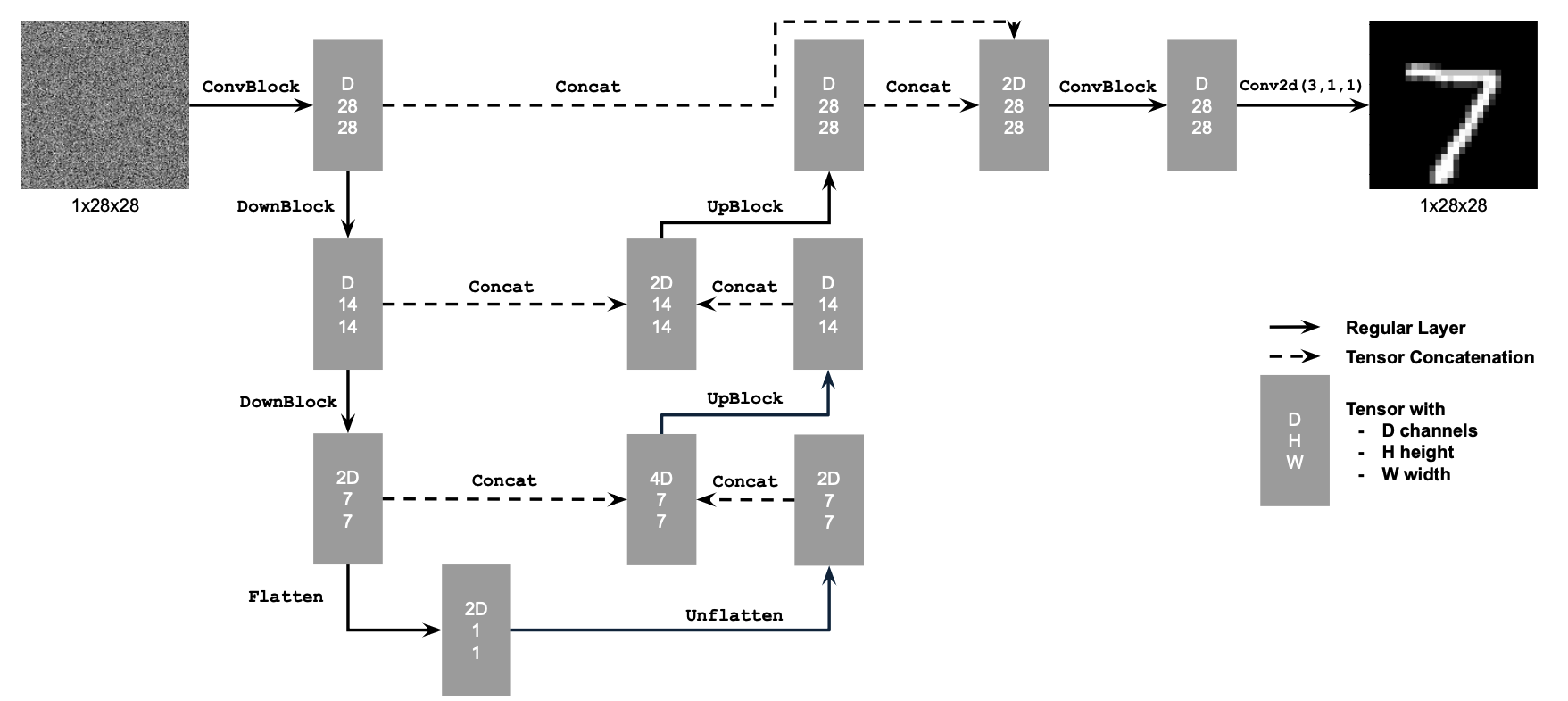
I began by creating a single-step denoising UNet. It takes in a noisy image, and predicts the original image by optimizing over an L2 loss between the original and outputted images. I followed the architecture shown below:
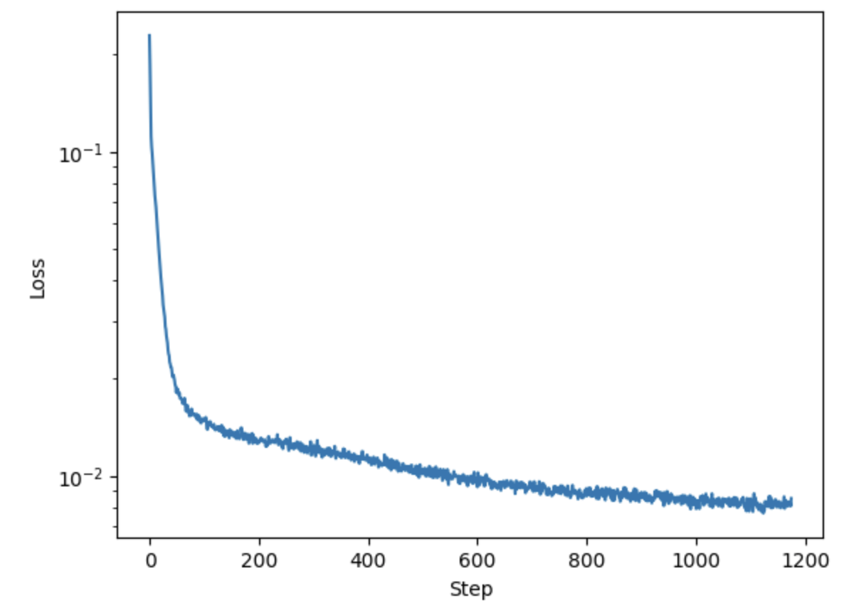
I trained this model using L2 loss function and Adam optimizer, the loss across iterations is shown below.
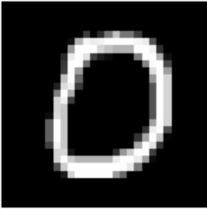
Here are the results shown after 1 epoch.
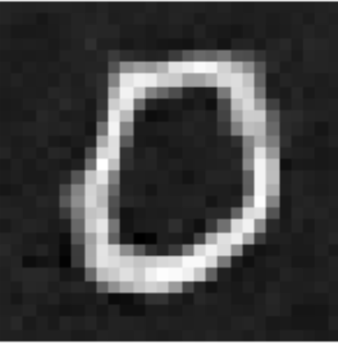

Here are the results shown after all 5 epochs.
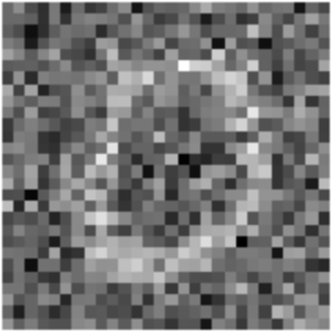
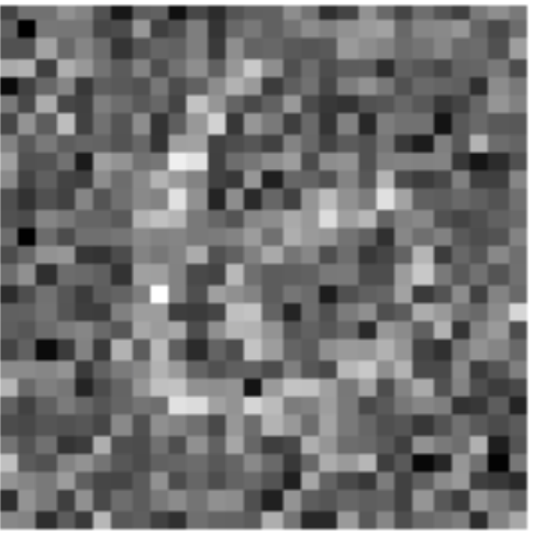
This model was trained with a σ value of 0.5, meaning the random noise generated is multipled by 0.5 before being added to the original image. We can vary this value, and test how well our model trained on 0.5 will work for other values.
Time Conditioned UNet
As we saw from the earlier results of image denoising, better results can be found by iteratively denoising an image. The following part is based off of the paper Denoising Diffusion Probabilistic Models (2020).
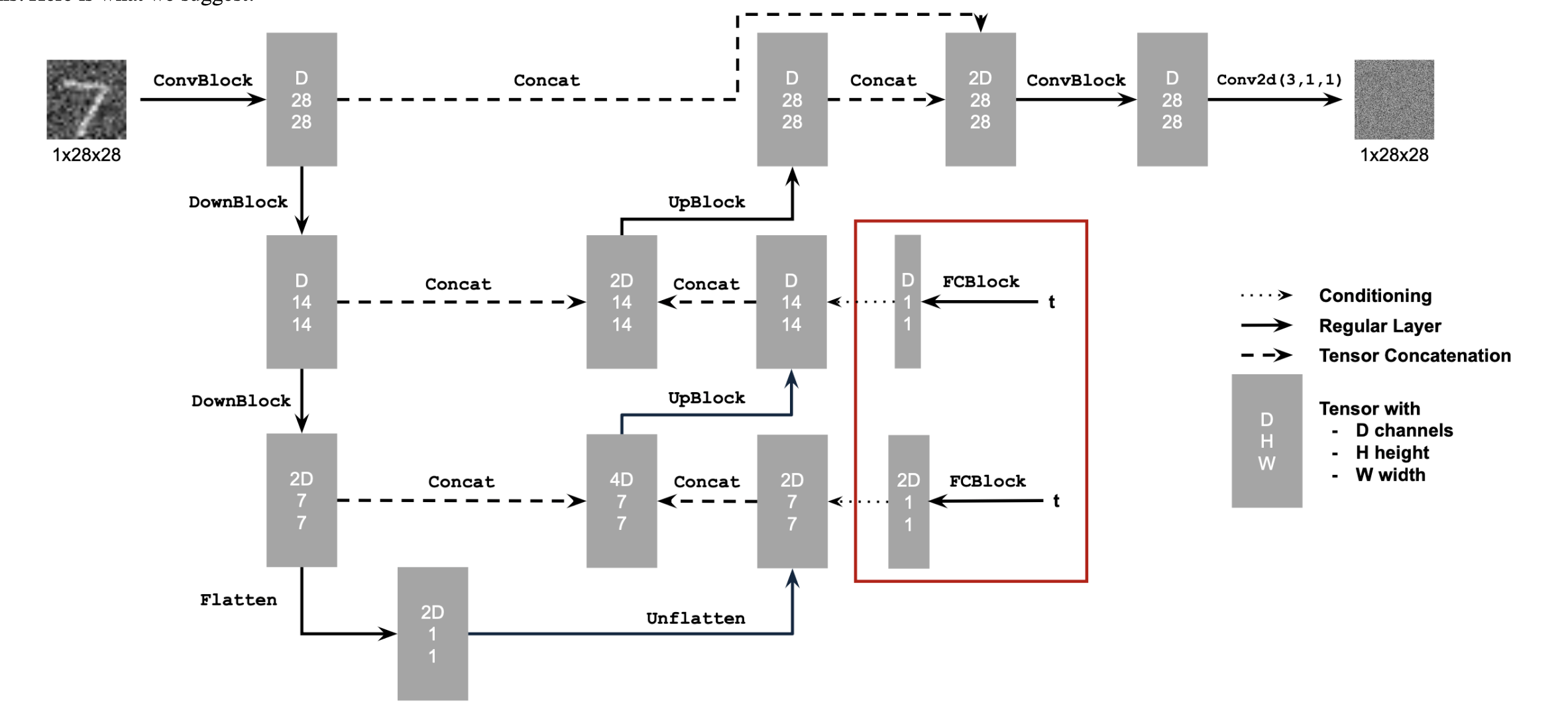
By adding a scalar t as a parameter to our model, we can condition it based off of the time, the method in which t is used is demonstrated in the image below.
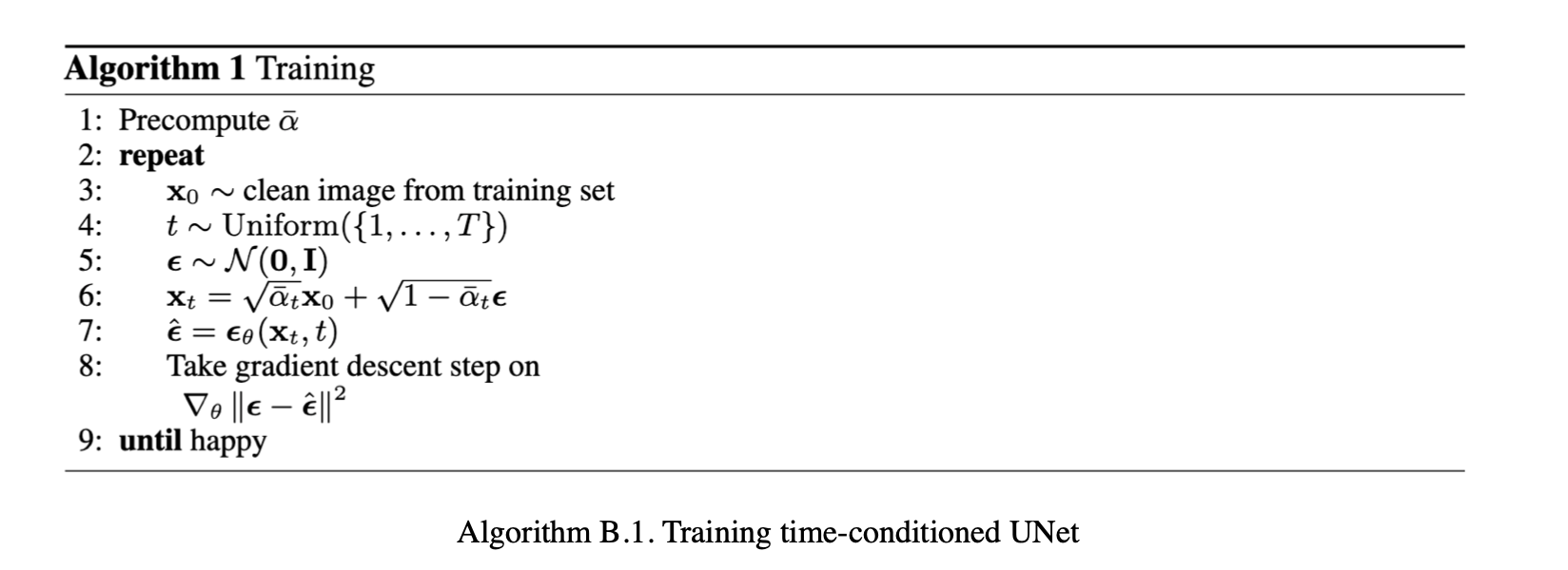
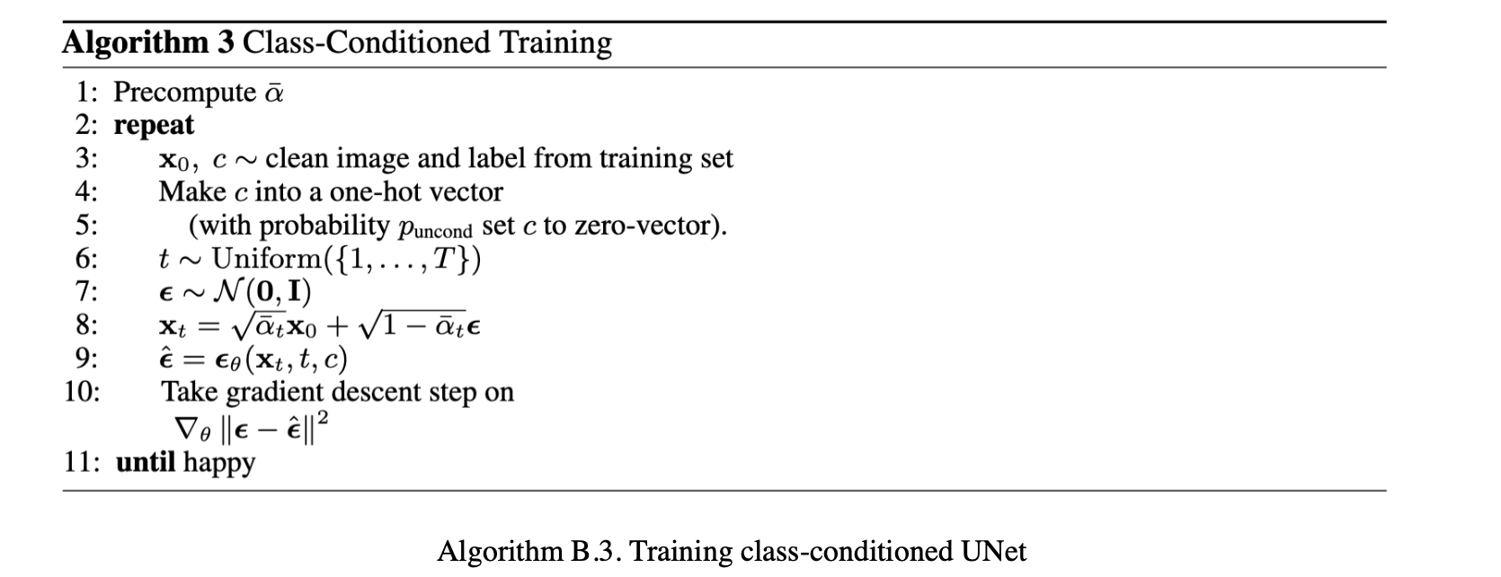
The training algorithm for this model is as follows:
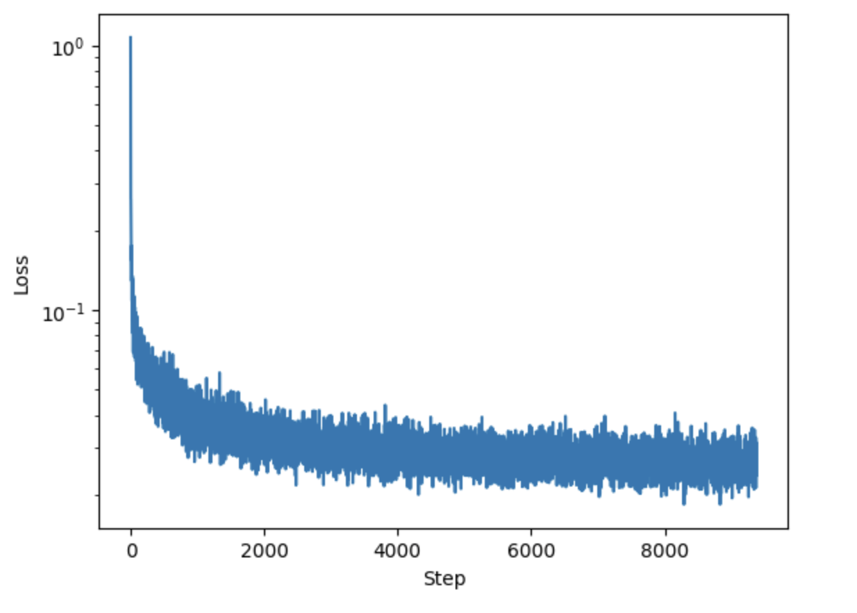
The loss curve for the training of this model is shown below:
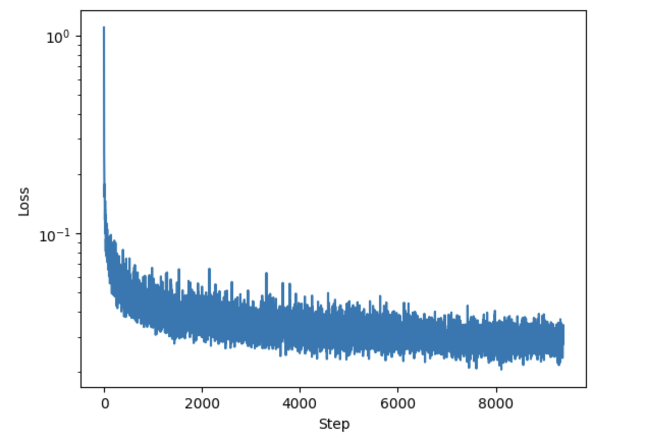
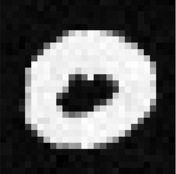
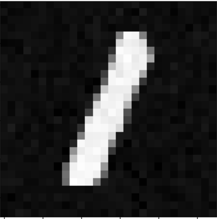
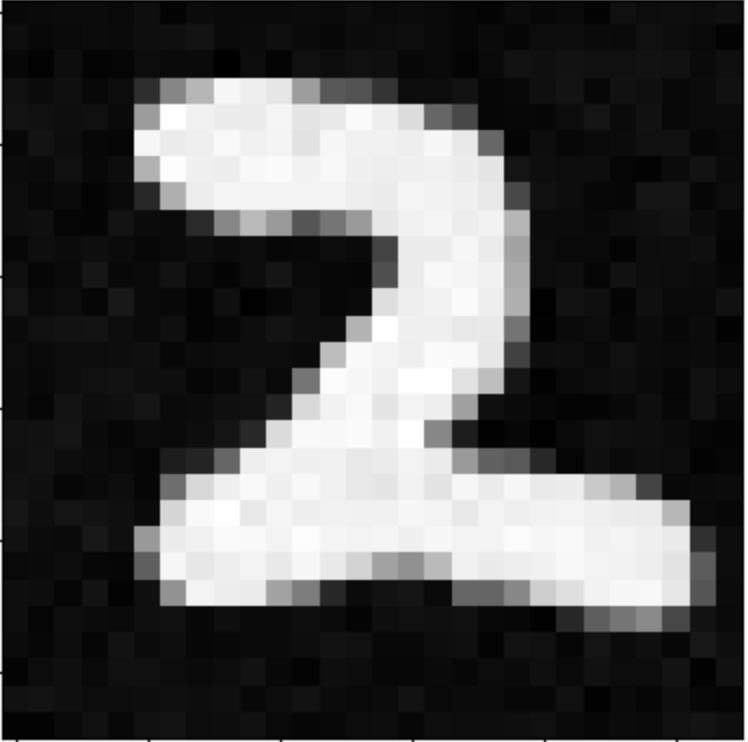
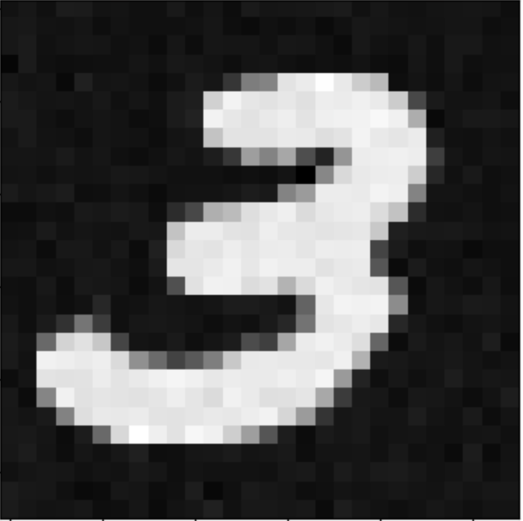
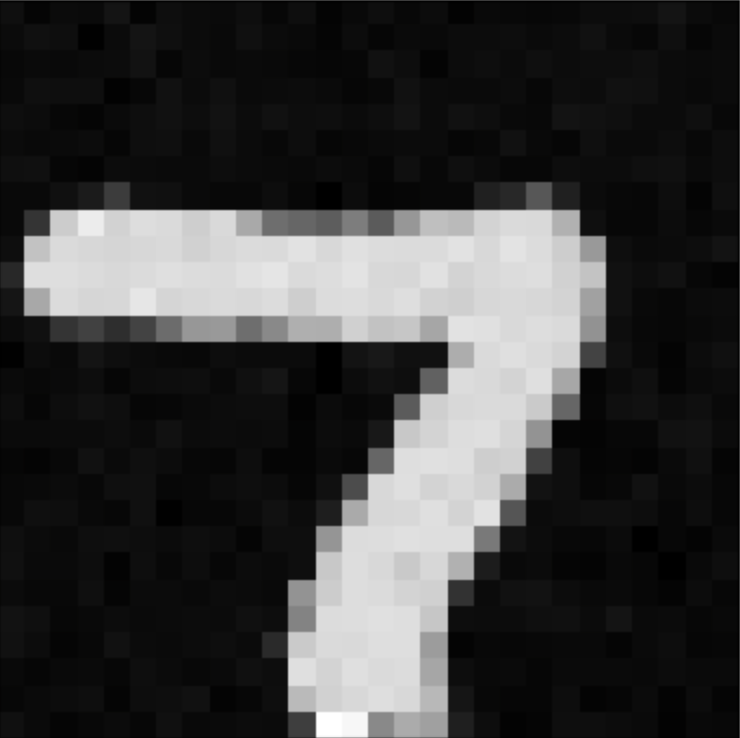
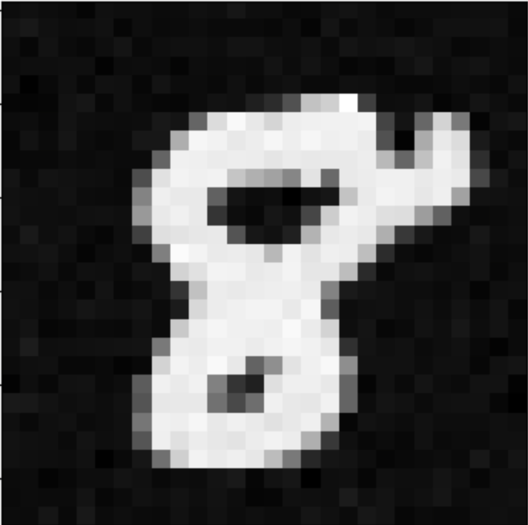
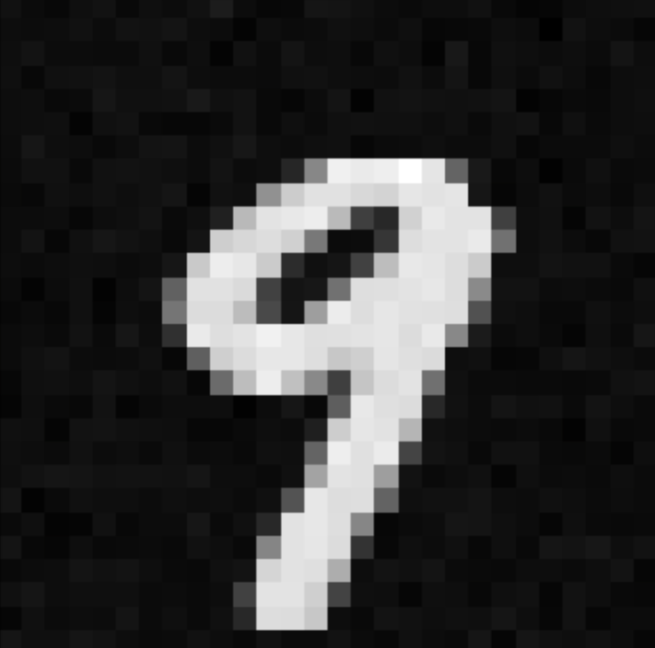
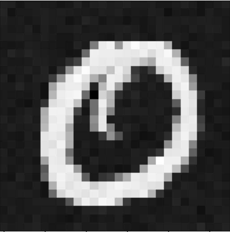
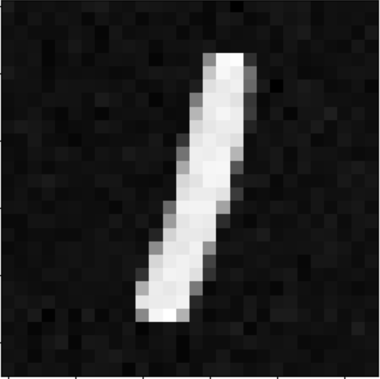
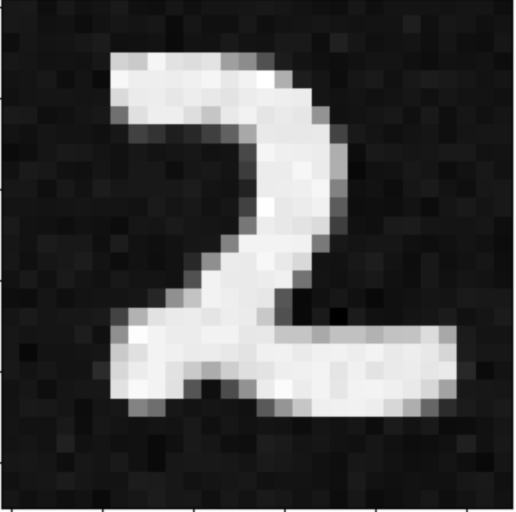
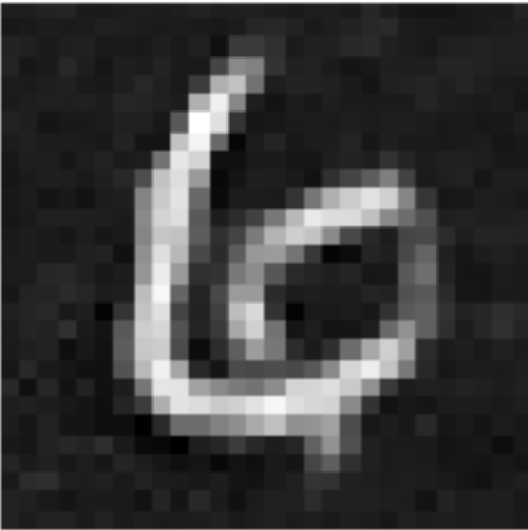
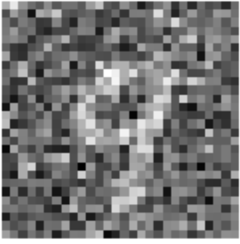
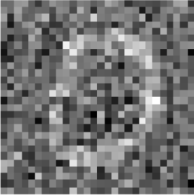
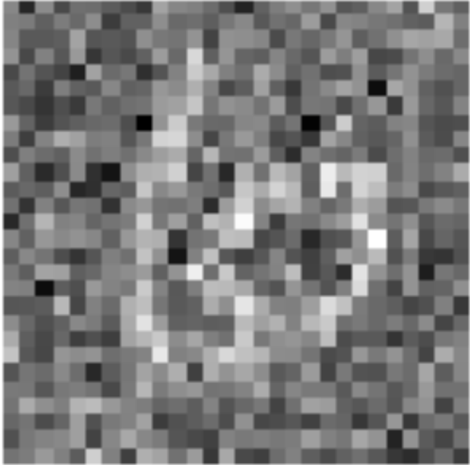
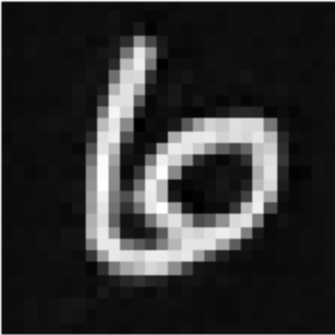
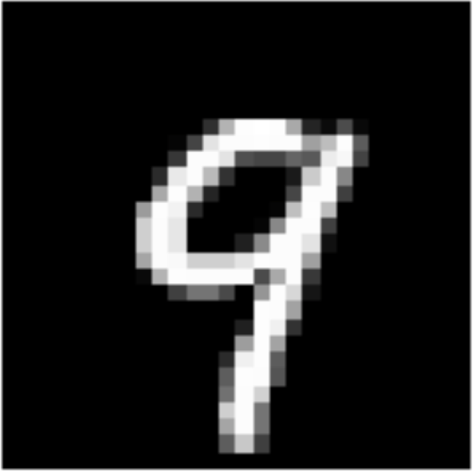
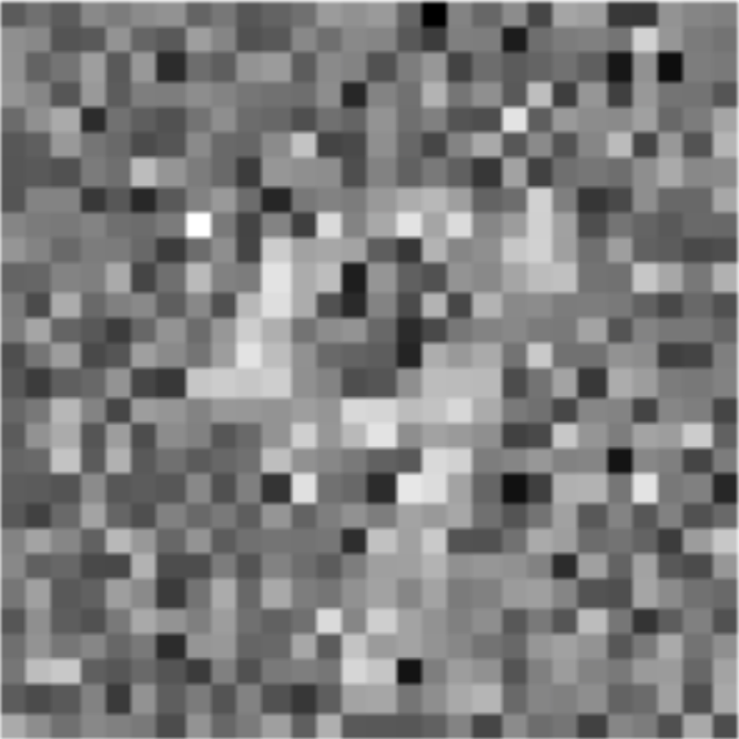
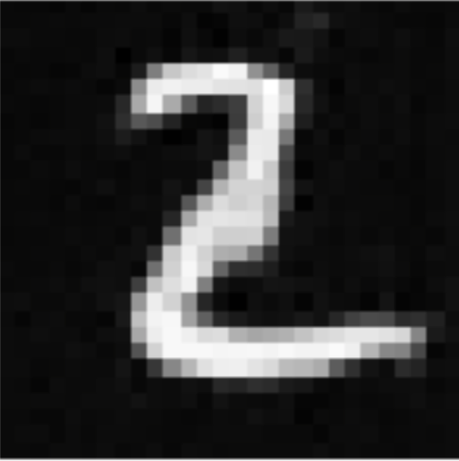
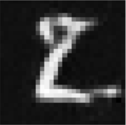
Results for this model shown at 5 epochs and 20 epochs are shown below:

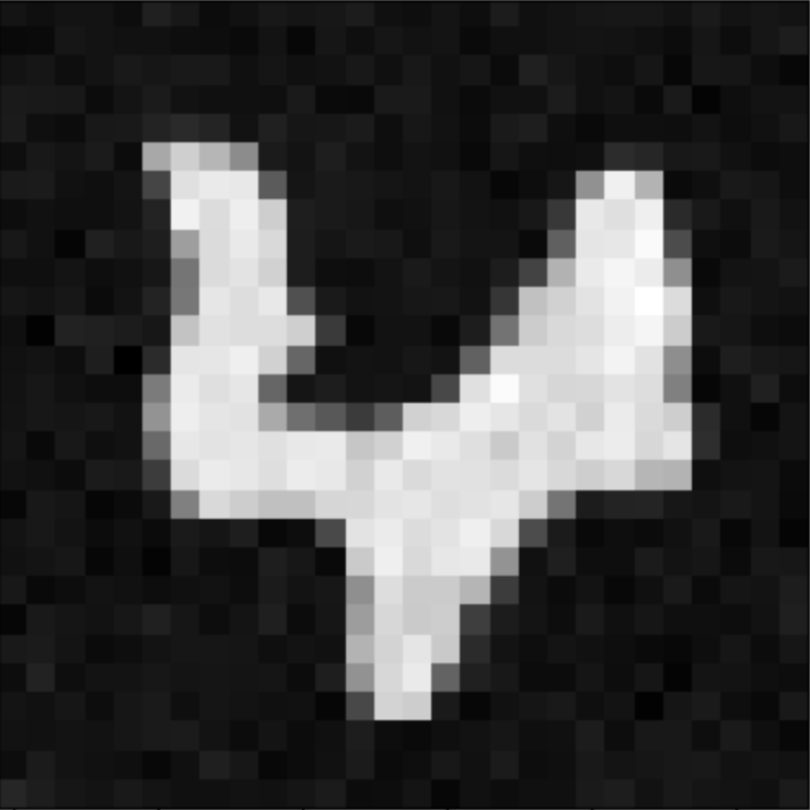
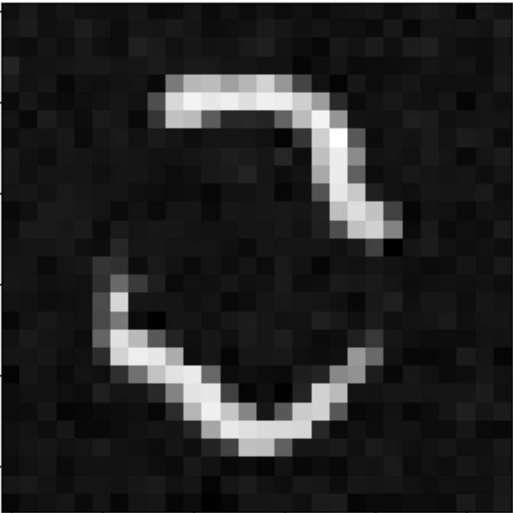
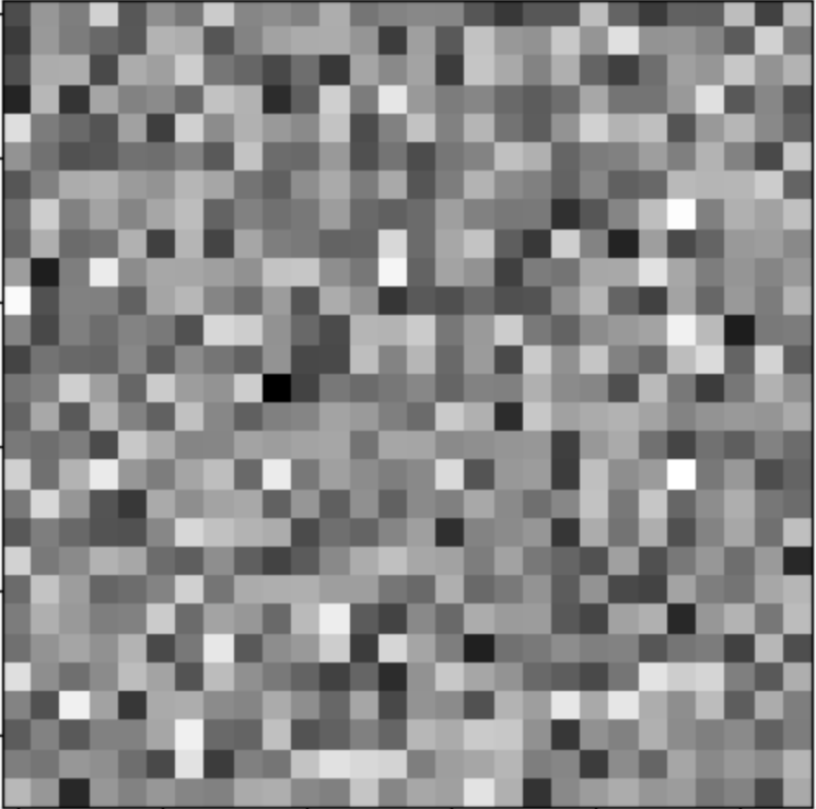
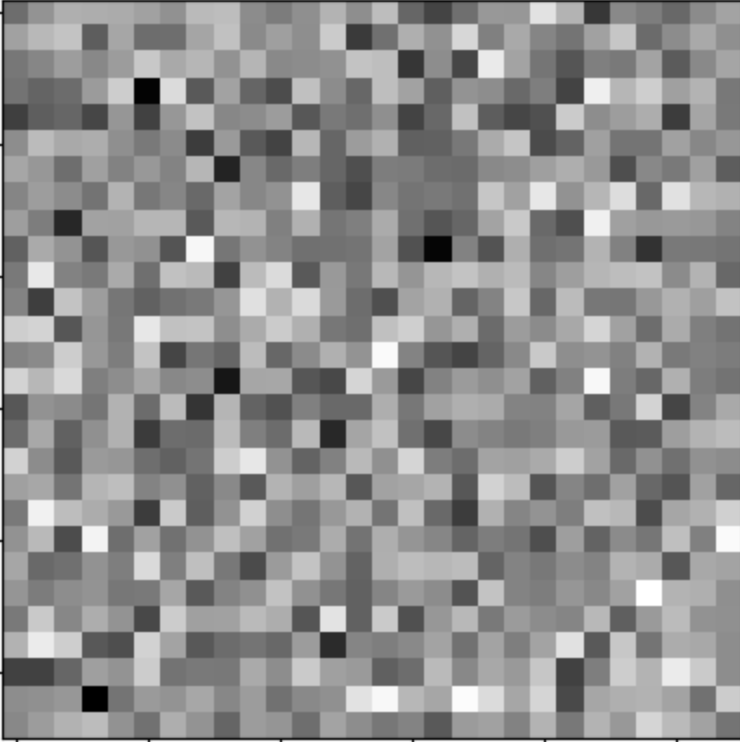
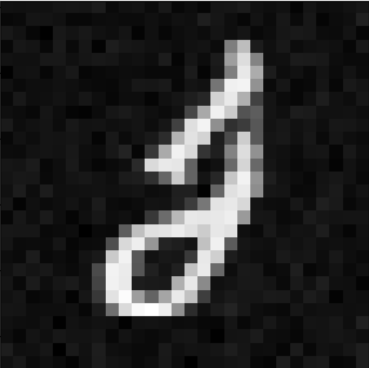
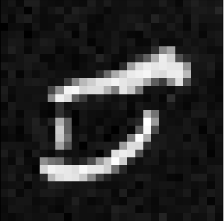
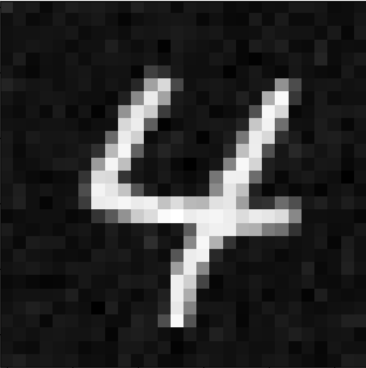
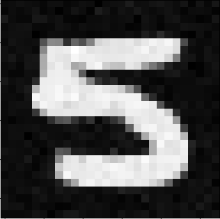
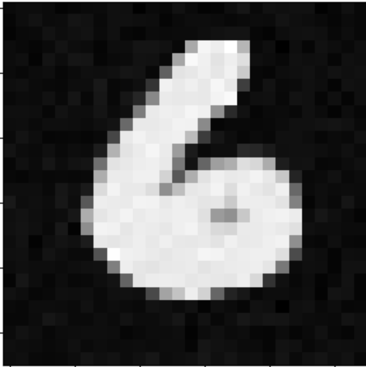
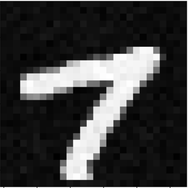
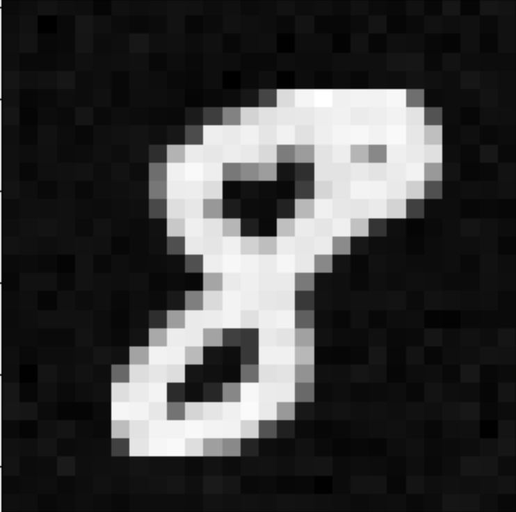
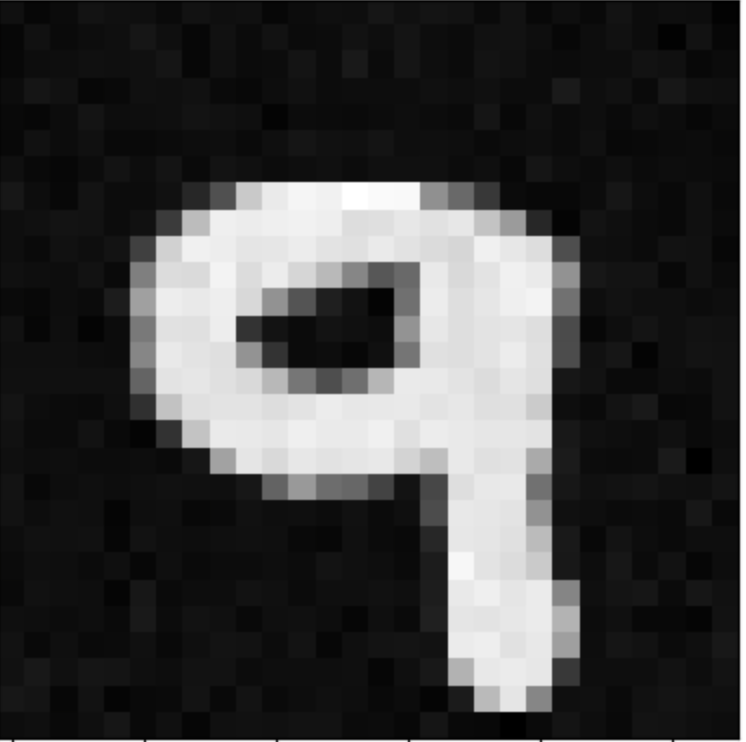
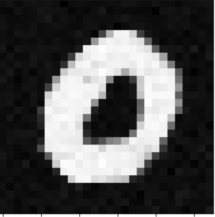
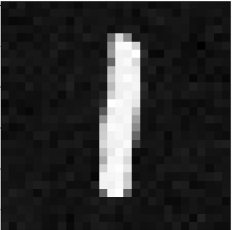
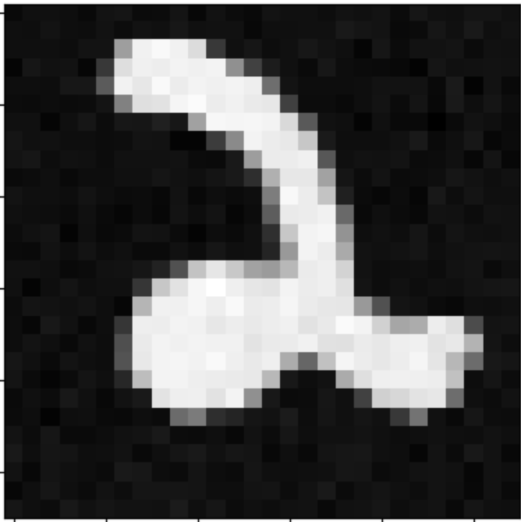
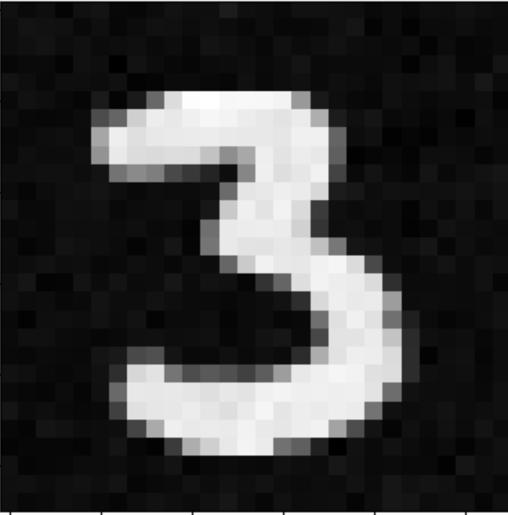
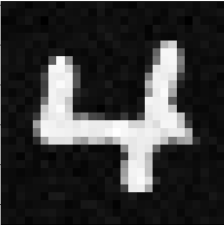
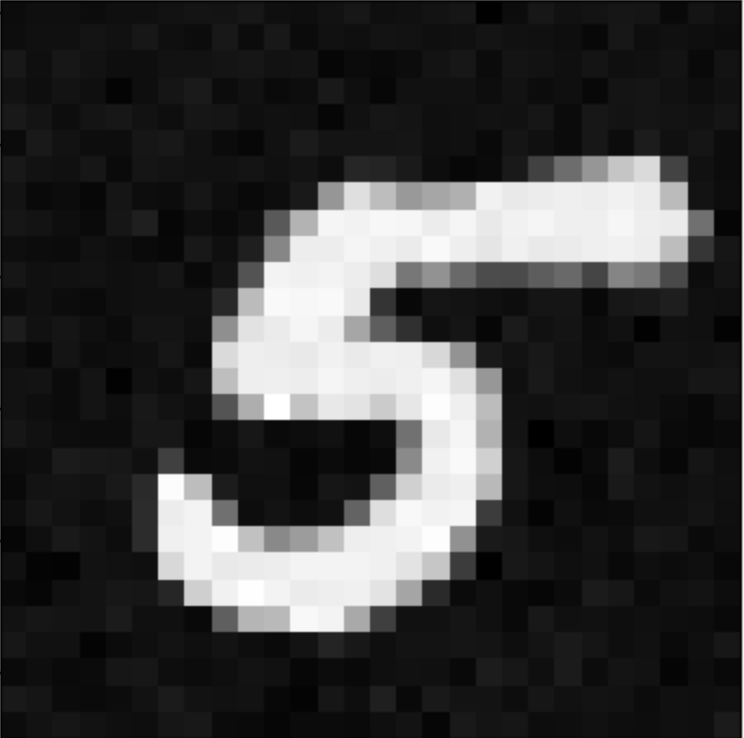
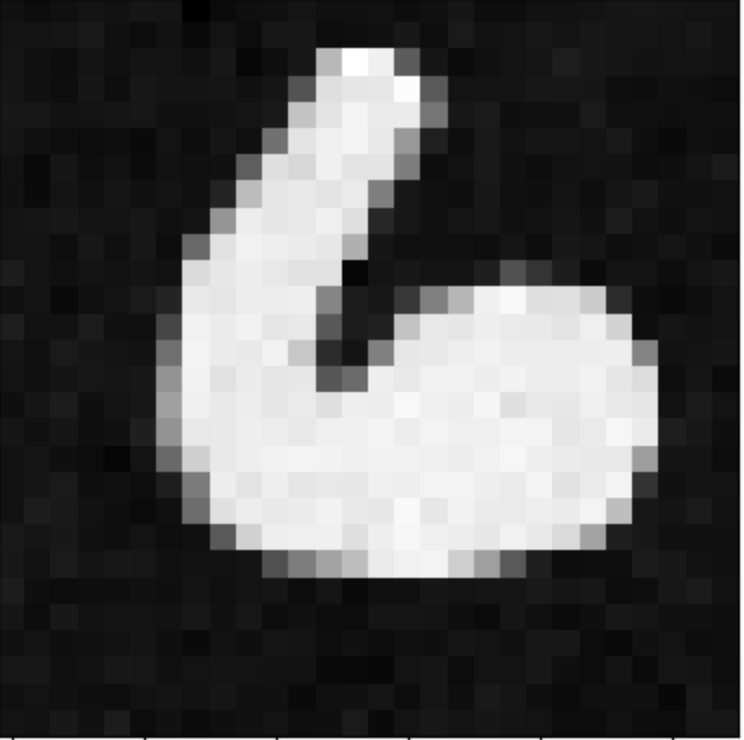
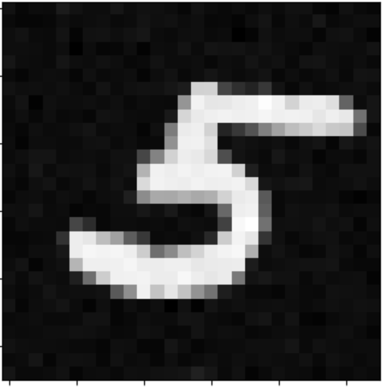
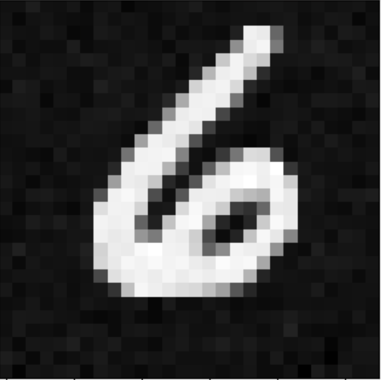
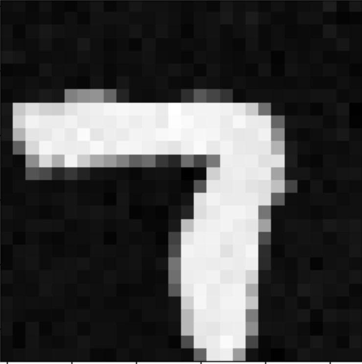
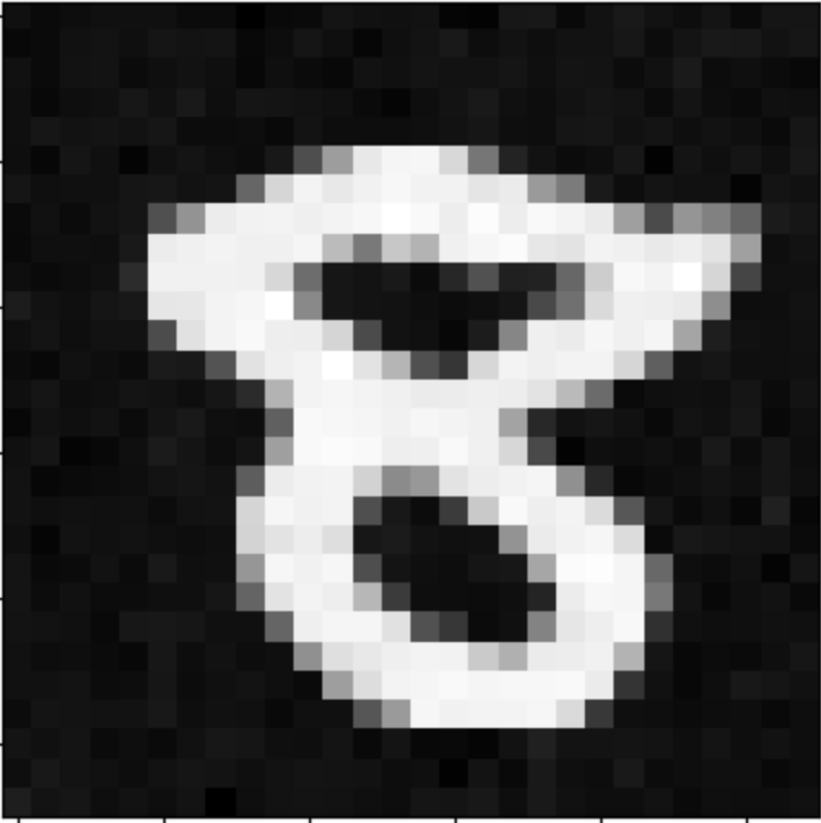
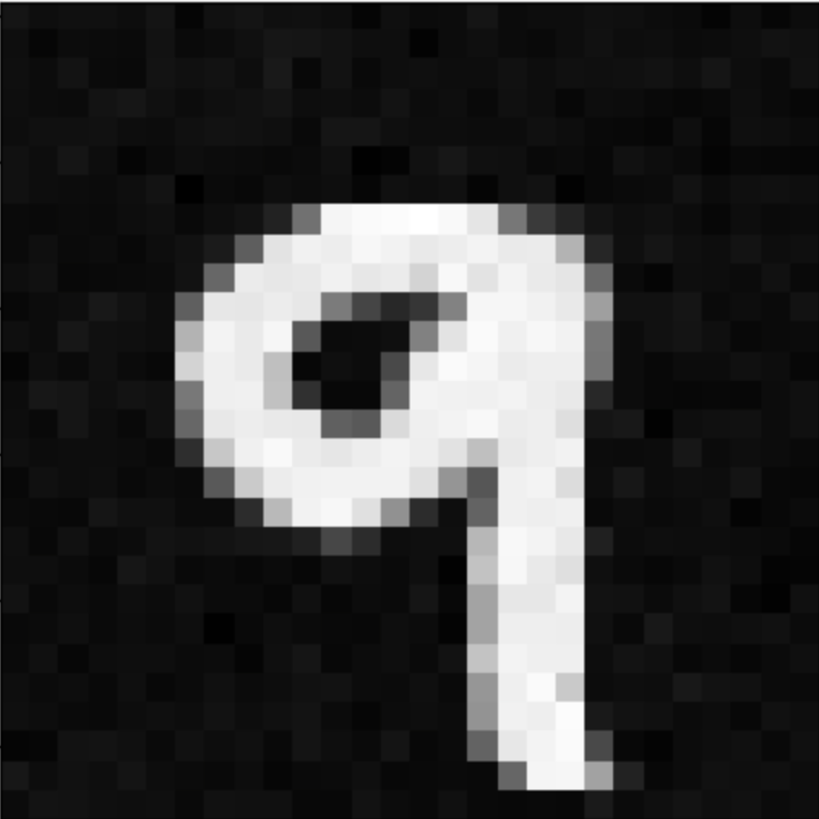
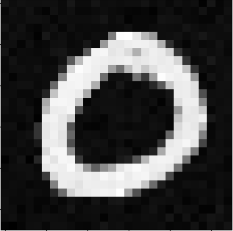
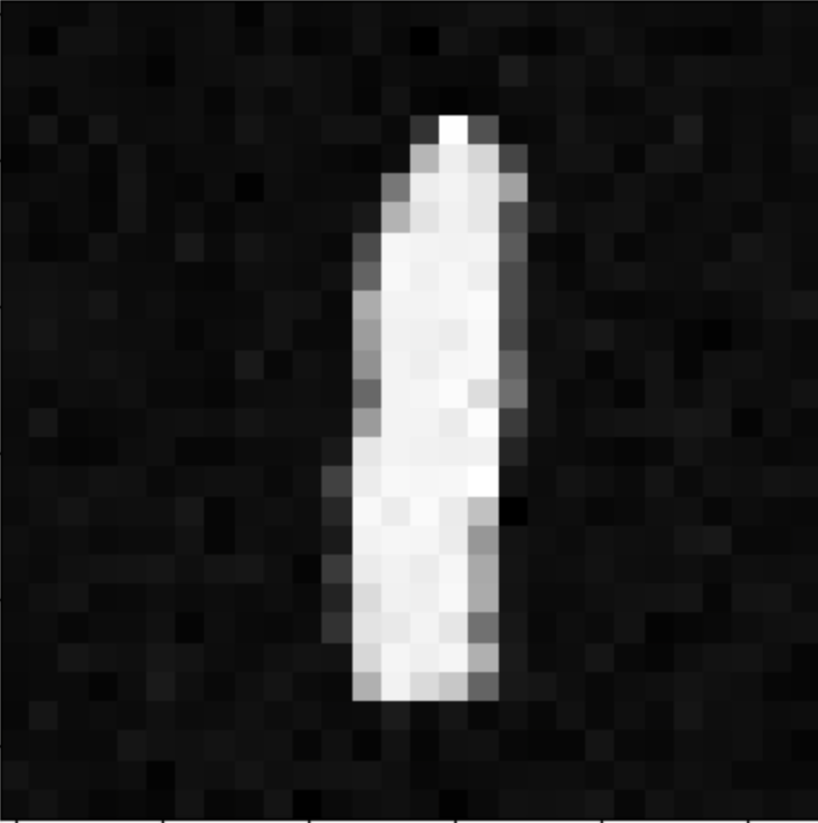
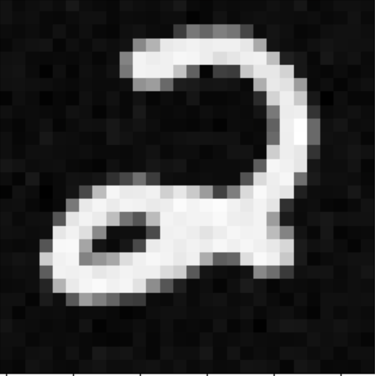
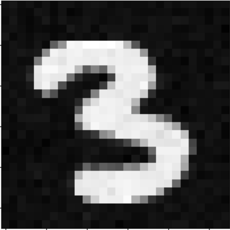
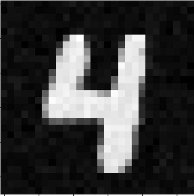
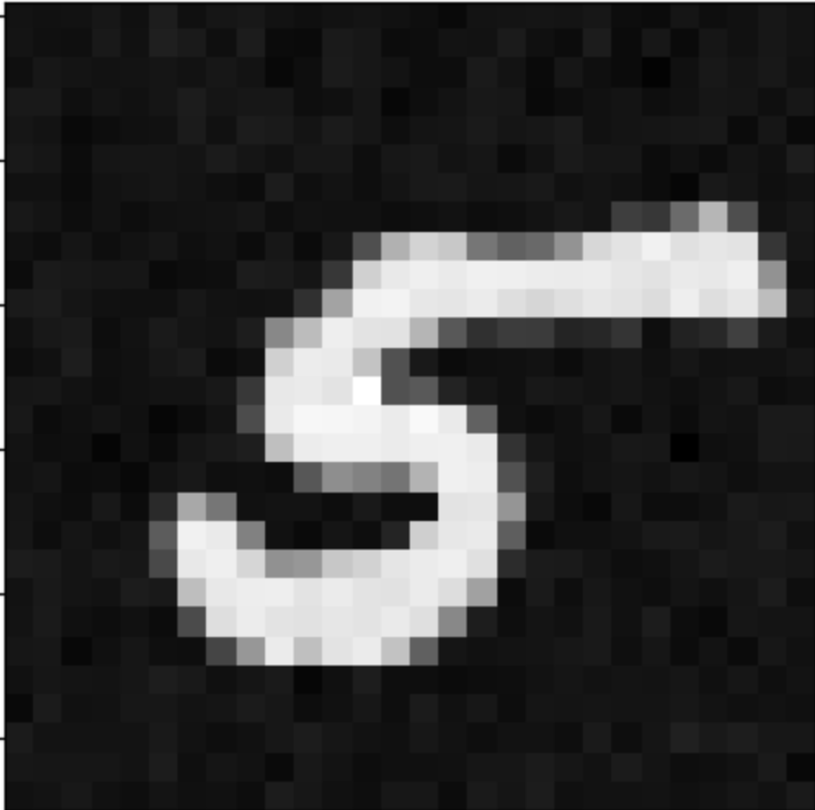
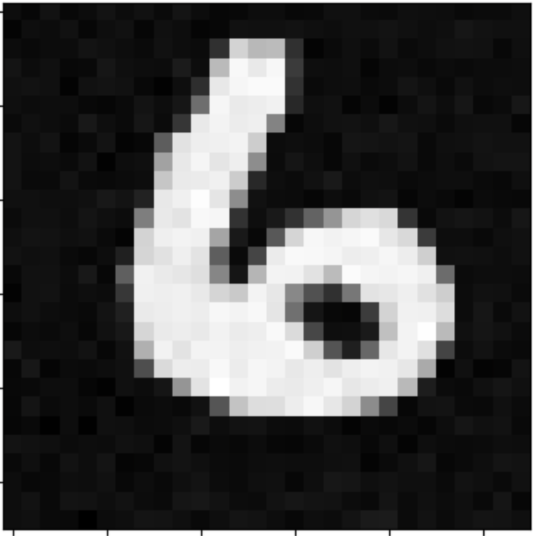
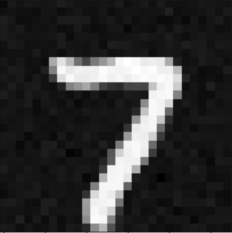
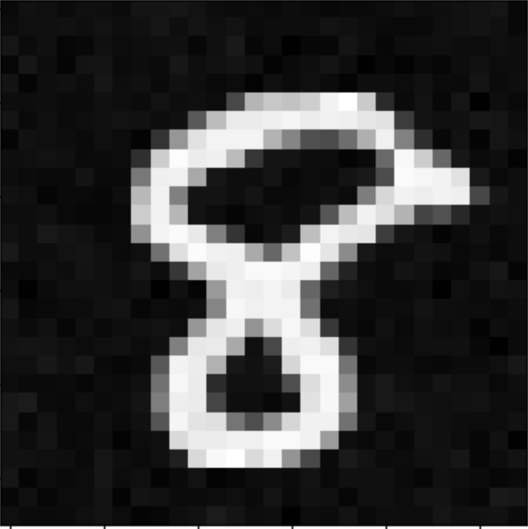
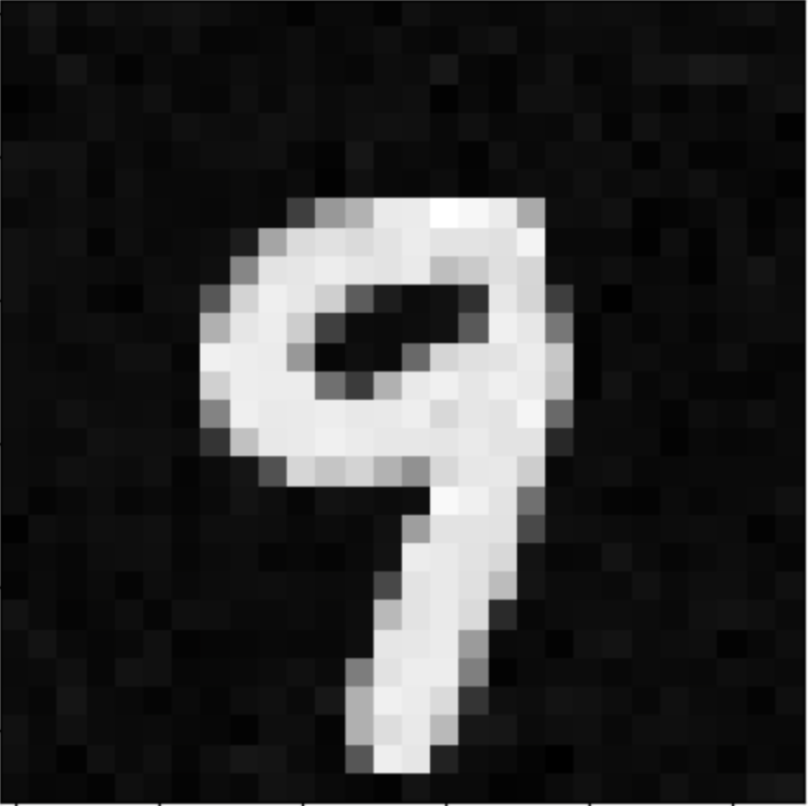
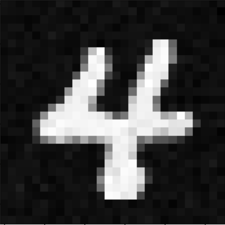
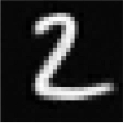
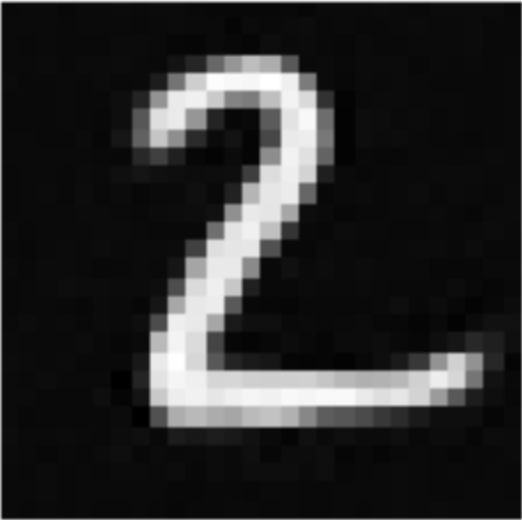
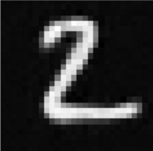
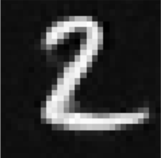
Class-Conditioned UNet
We can improve on these results by conditioning the UNet on the digits 0-9. This involves training on the digit numbers itself with each of the images, and passing this as a parameter through the model as well.
The loss curve for the training of this model is shown below:
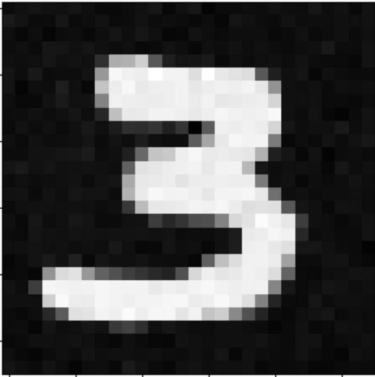
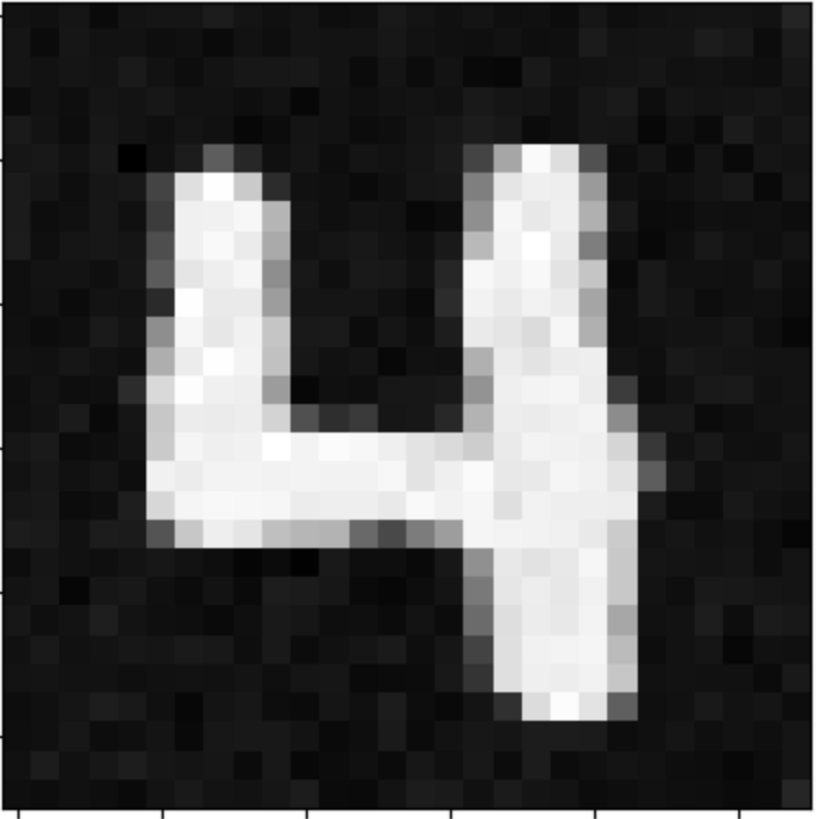
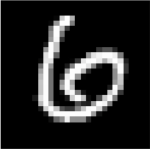
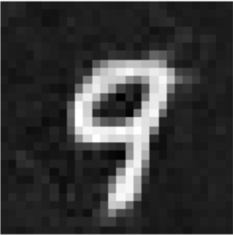
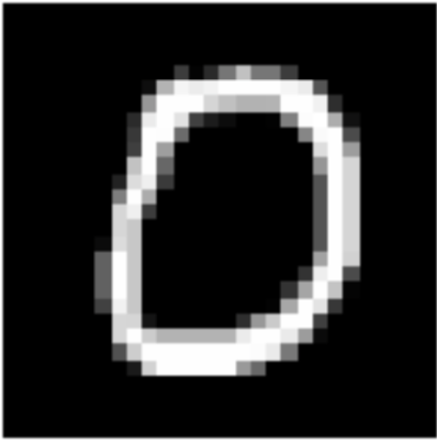
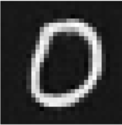
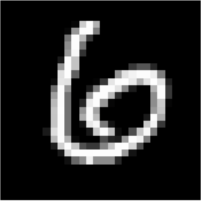
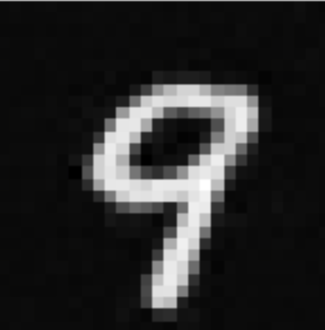
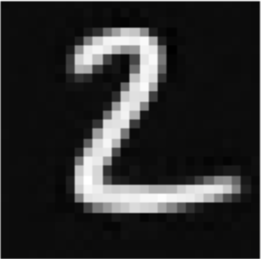
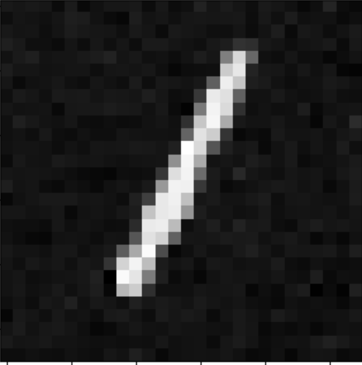
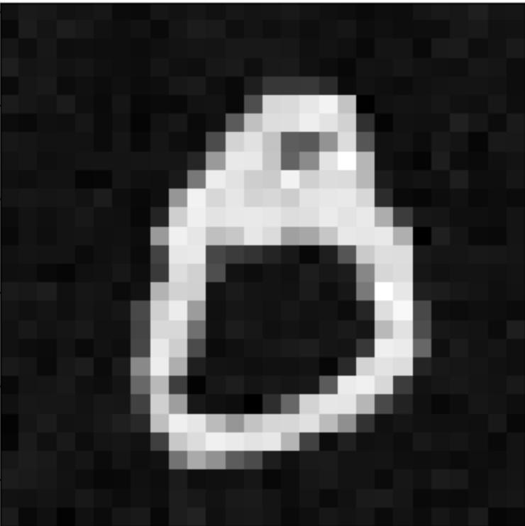
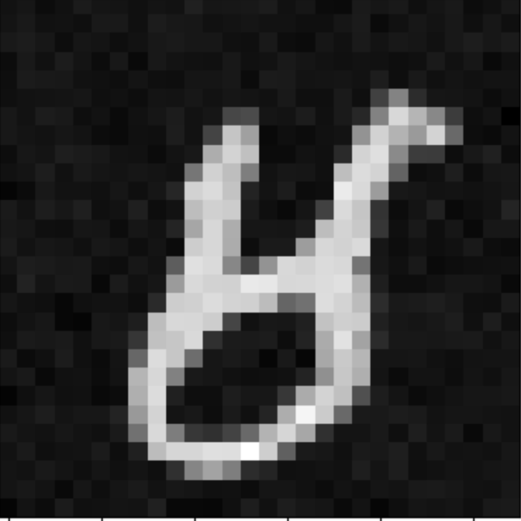
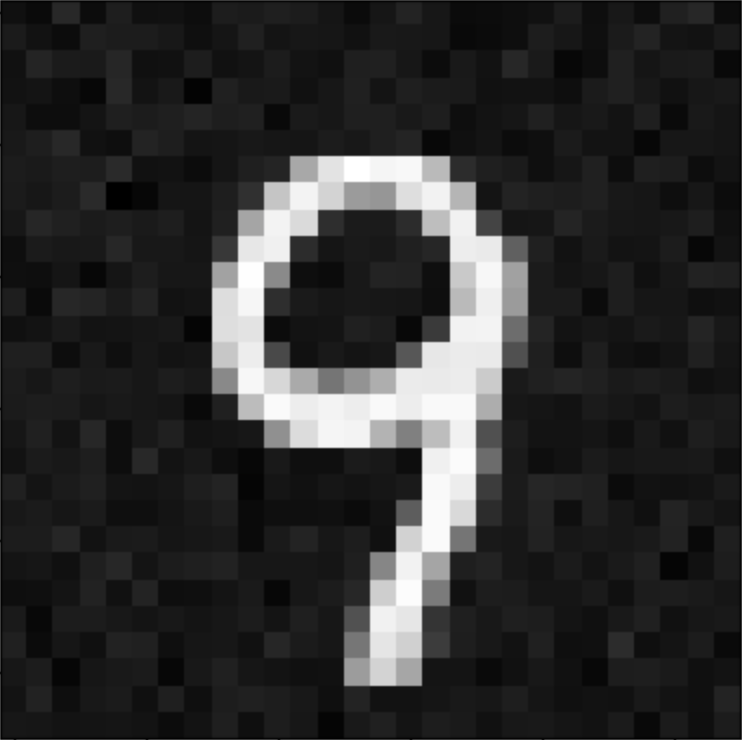
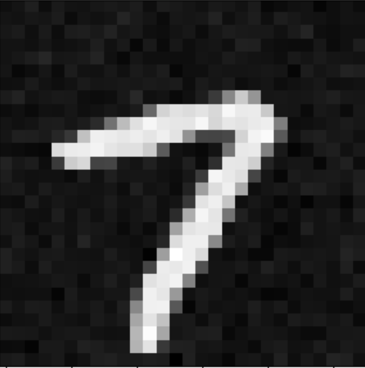
Results of the model shown at 5 epochs is shown below.
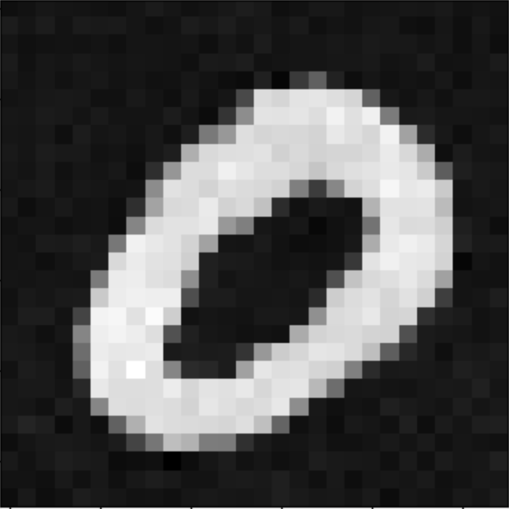
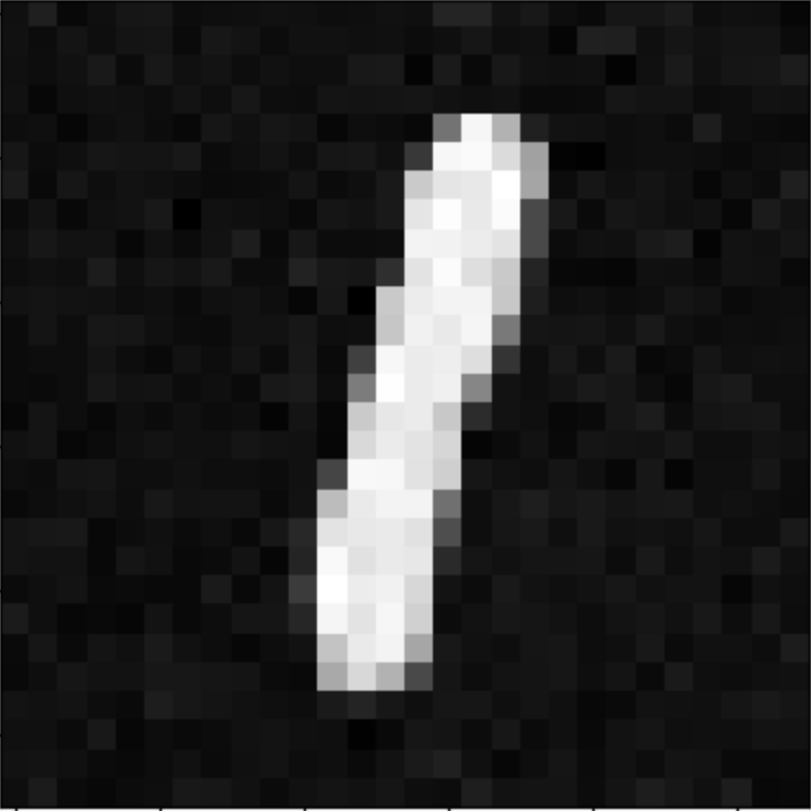
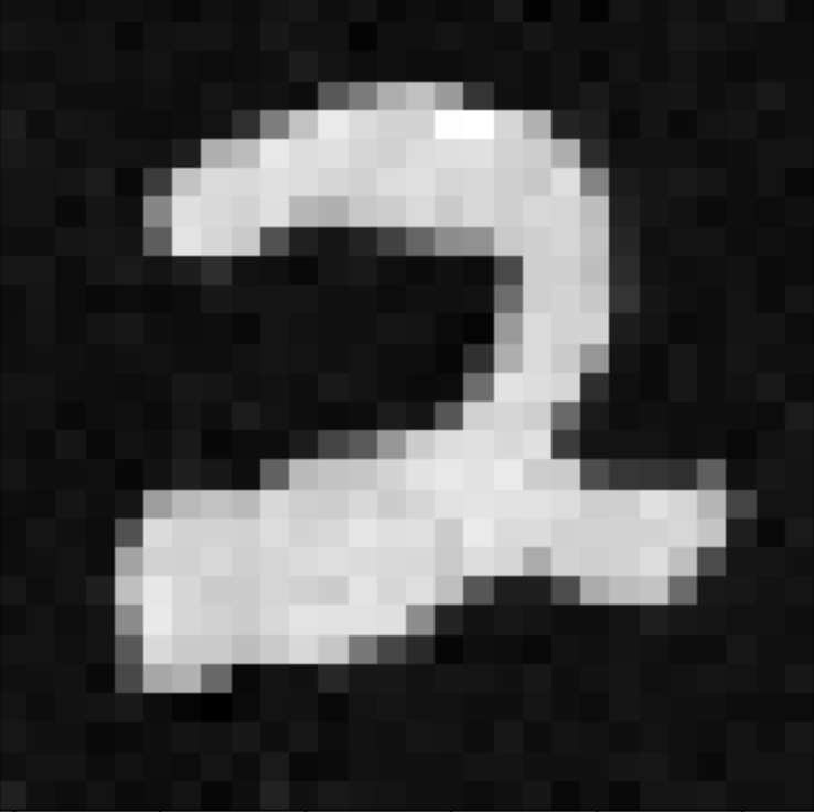
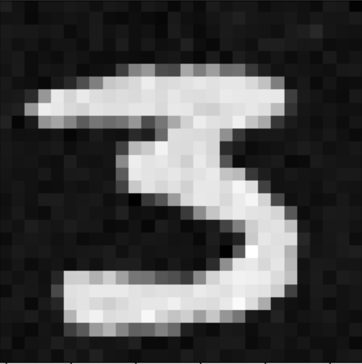
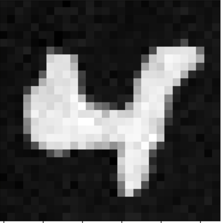
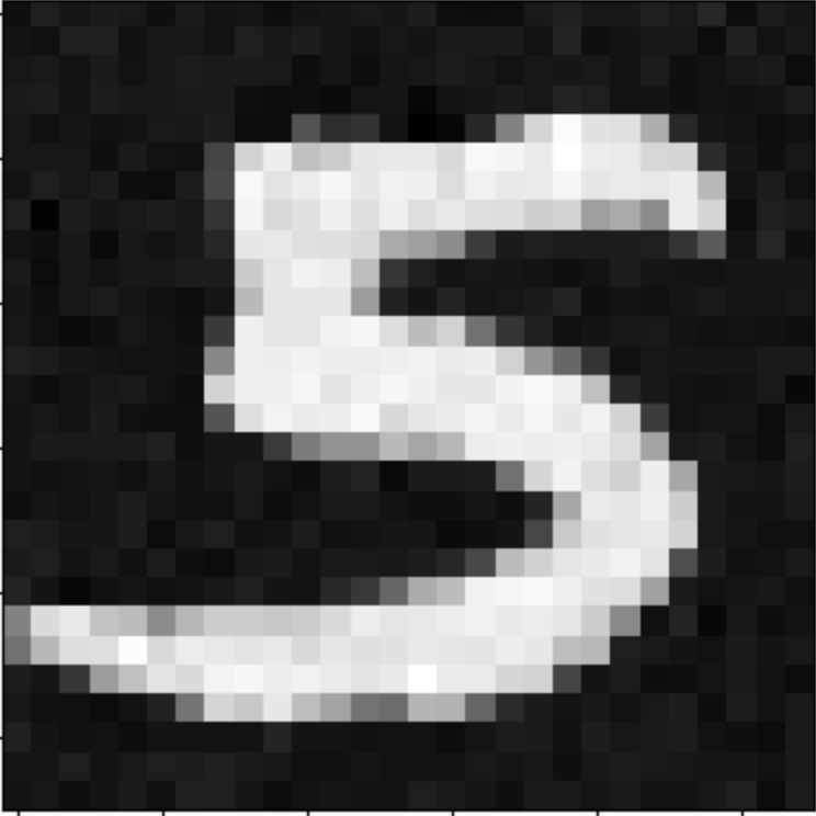
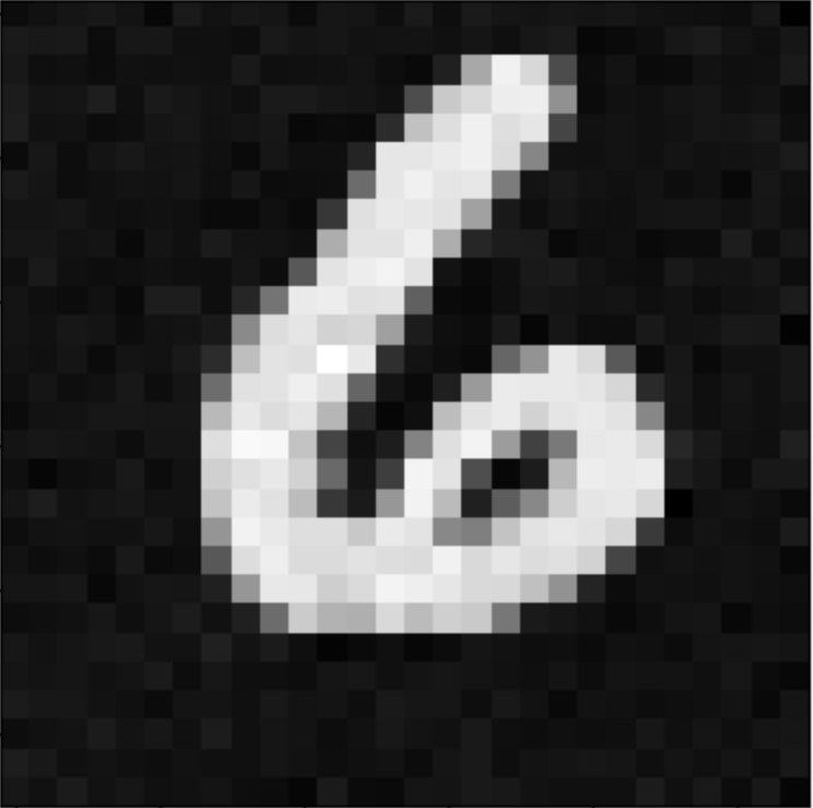
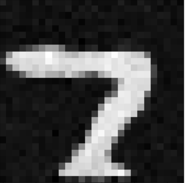
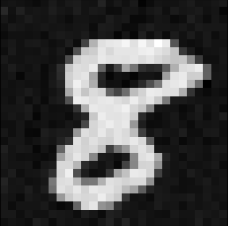
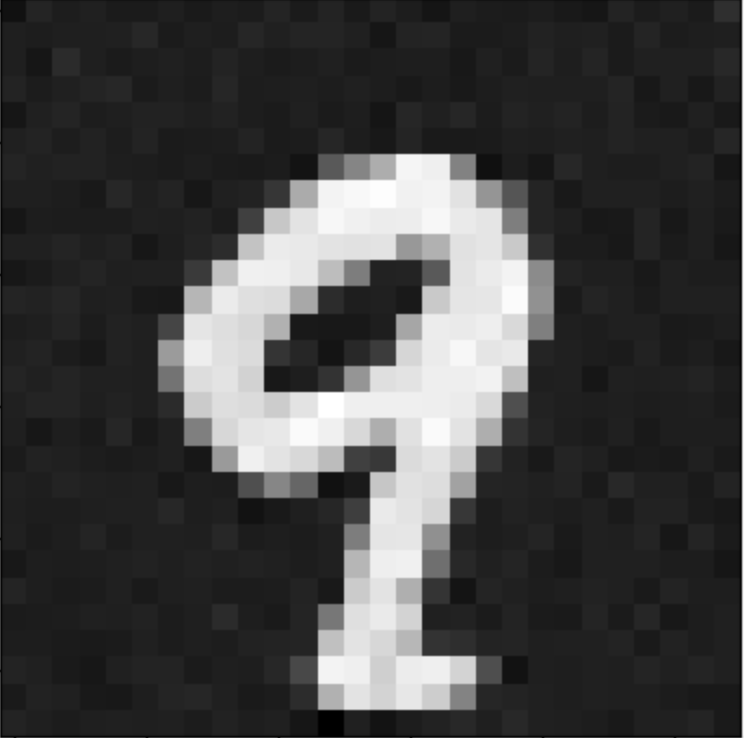
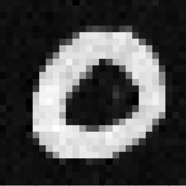
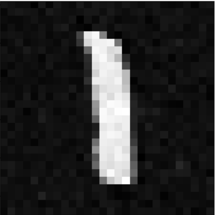
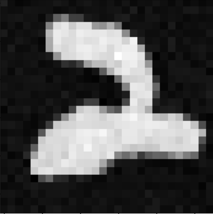
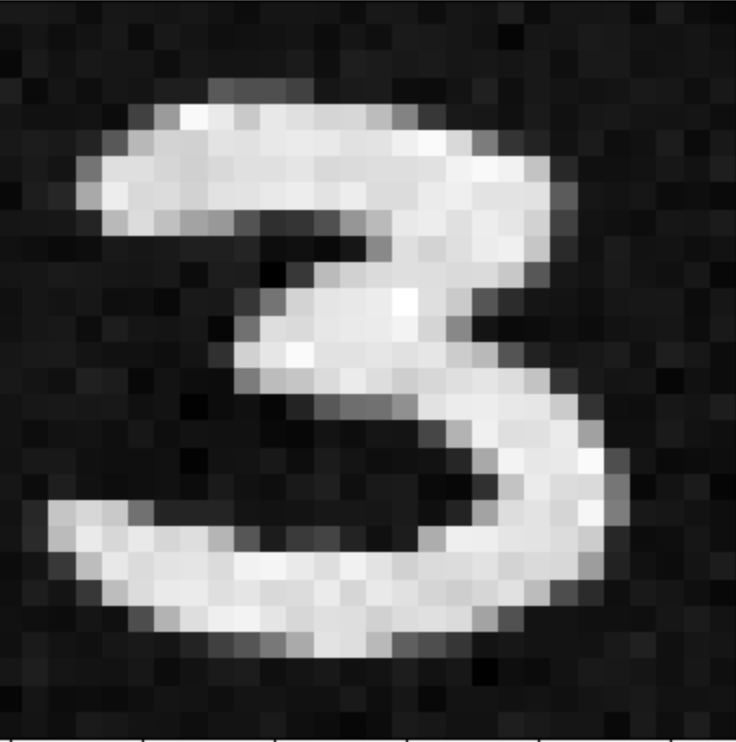
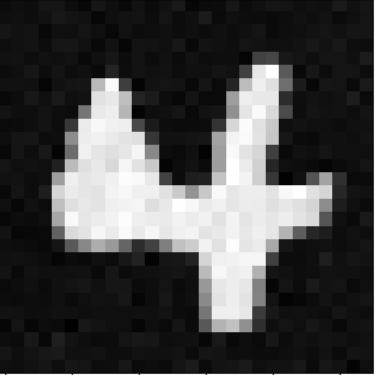
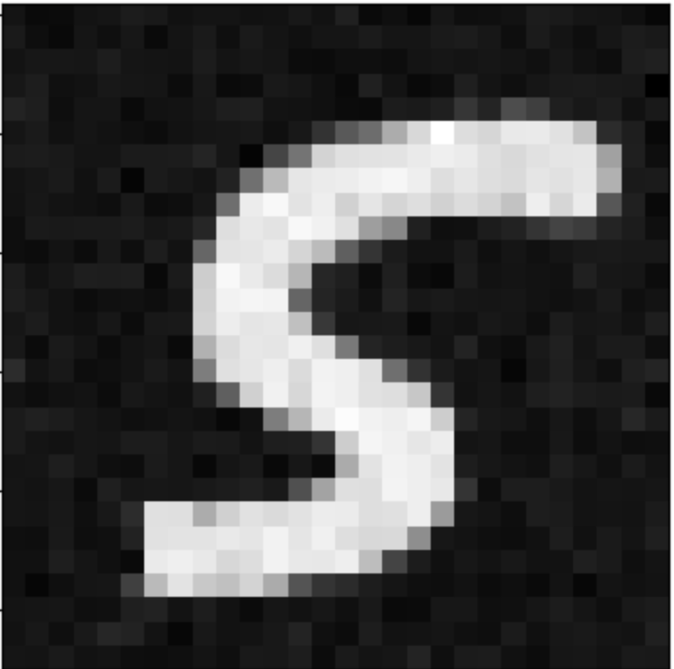
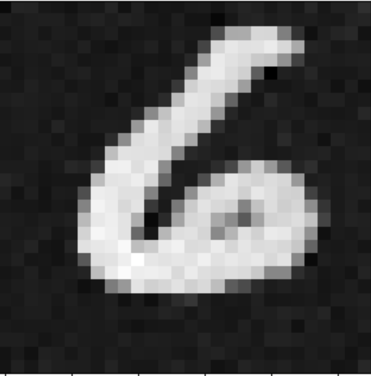
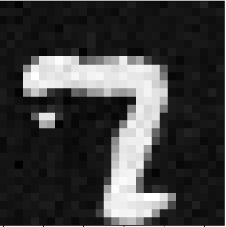
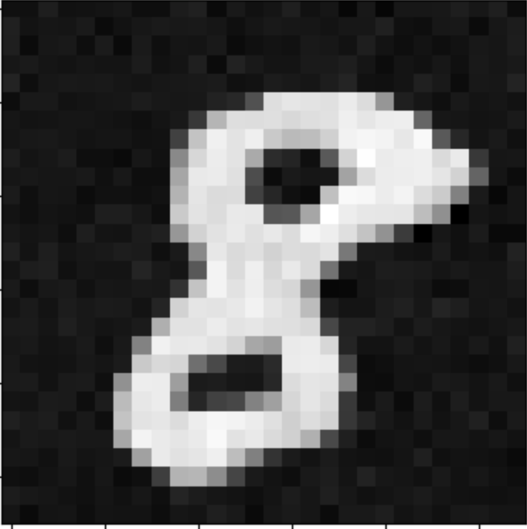
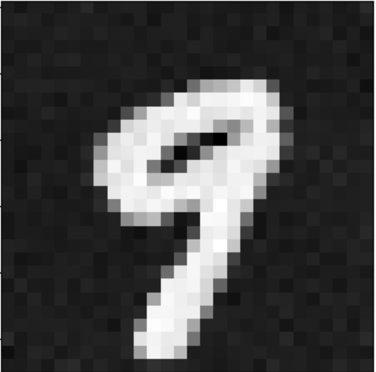
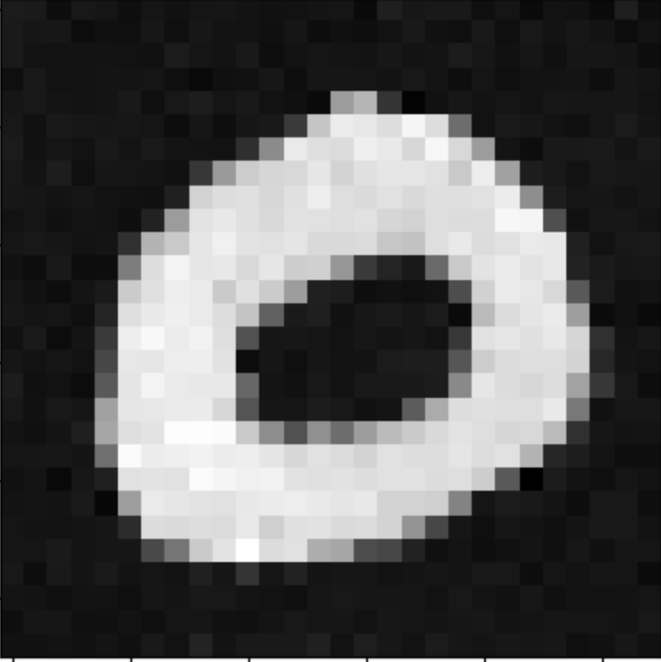
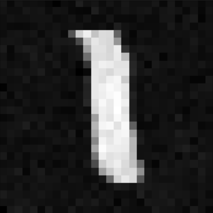
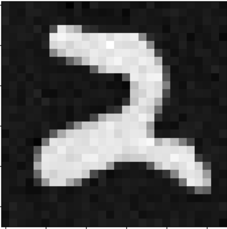
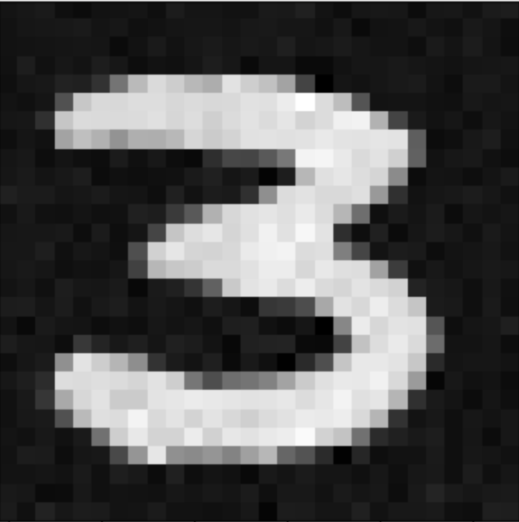
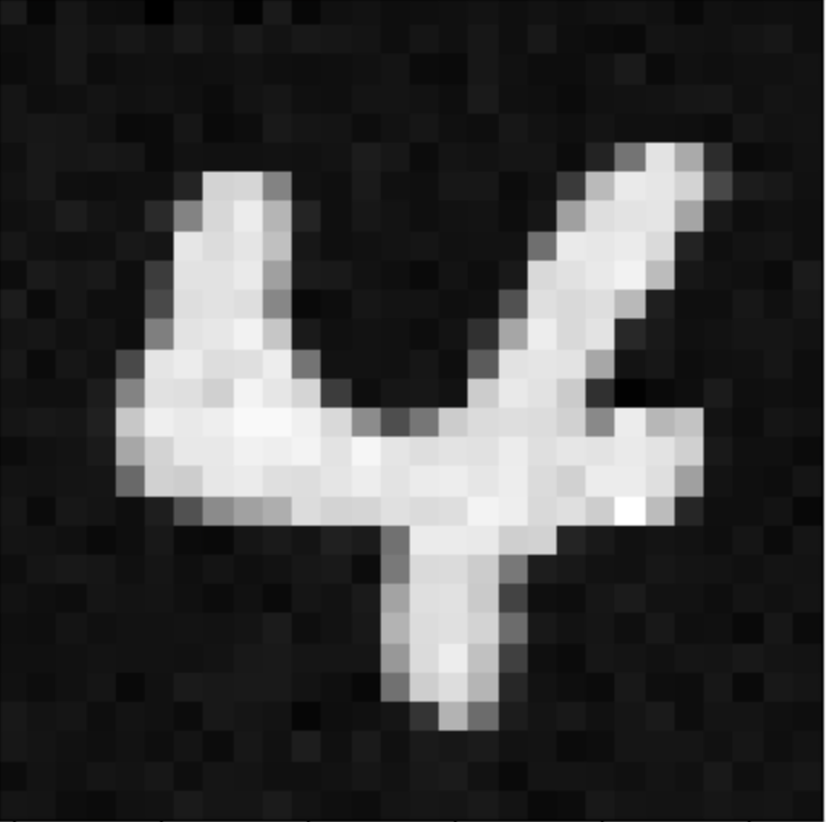
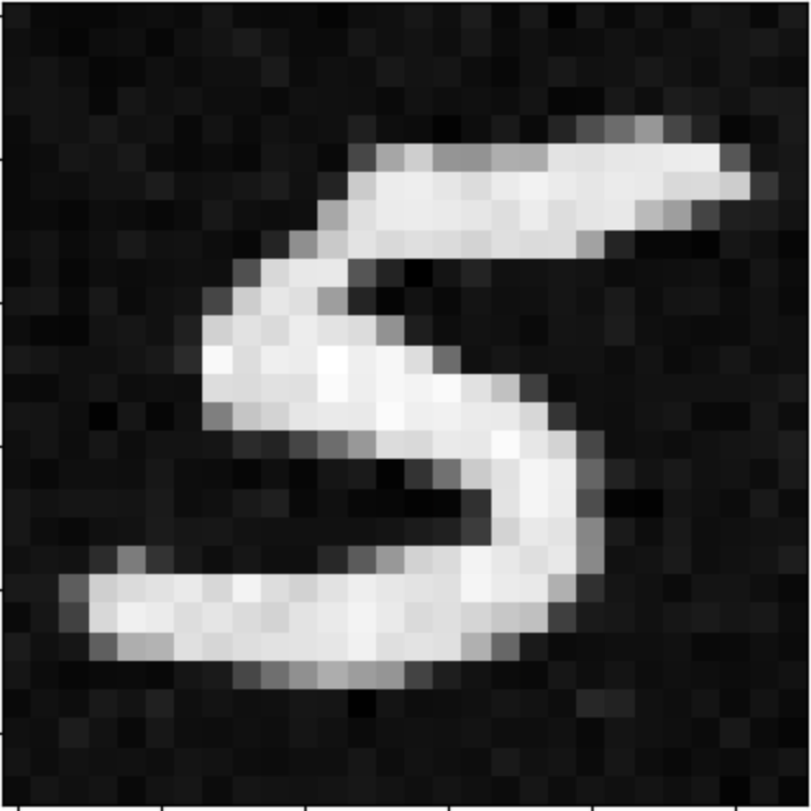
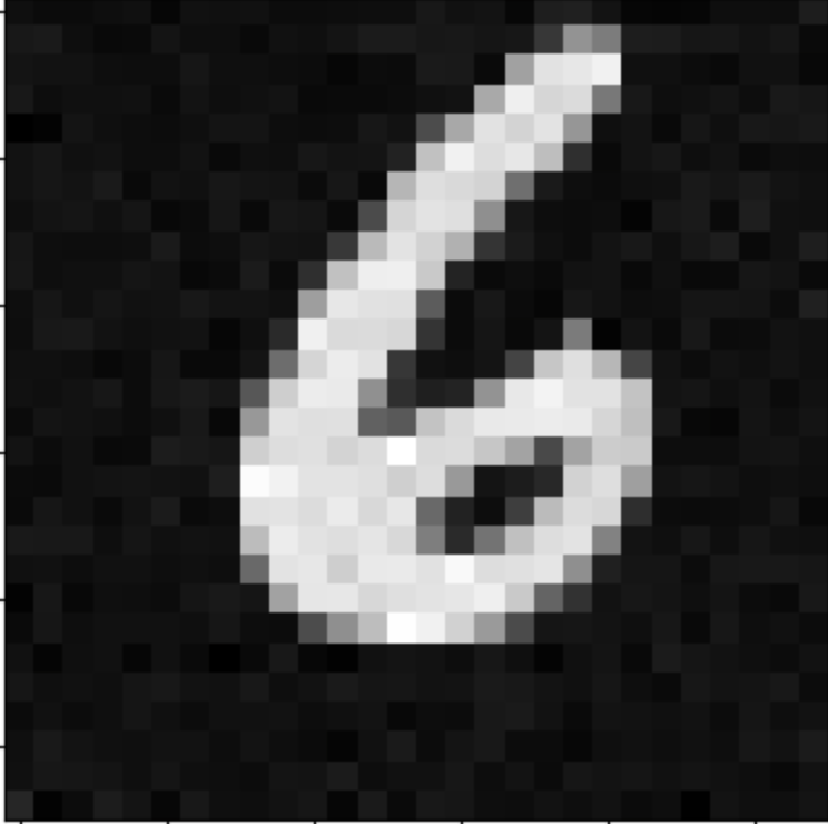
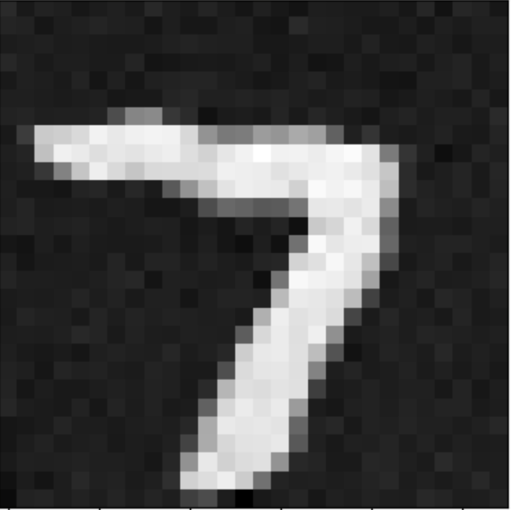
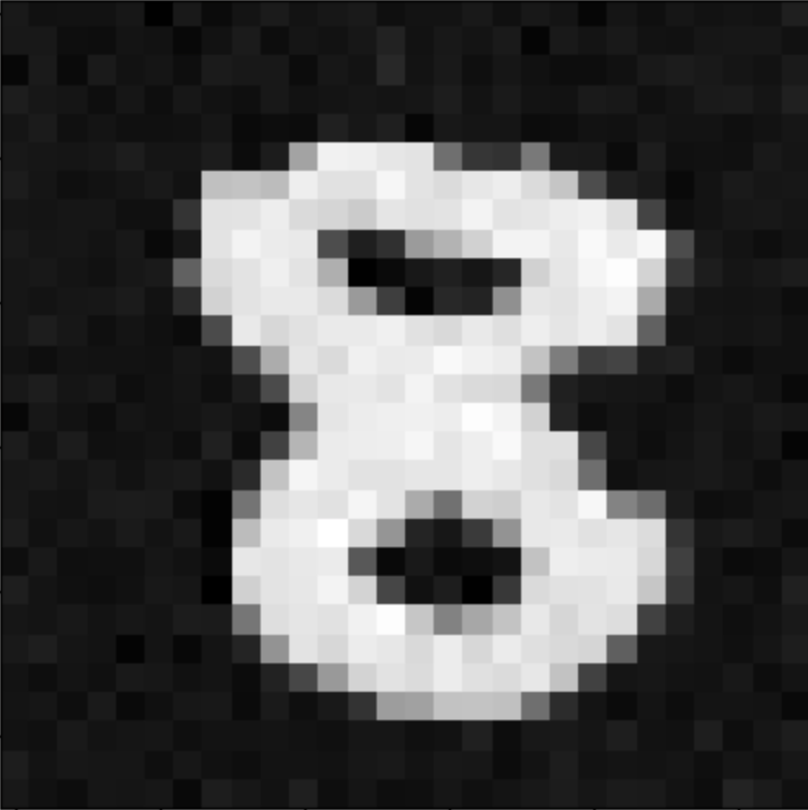
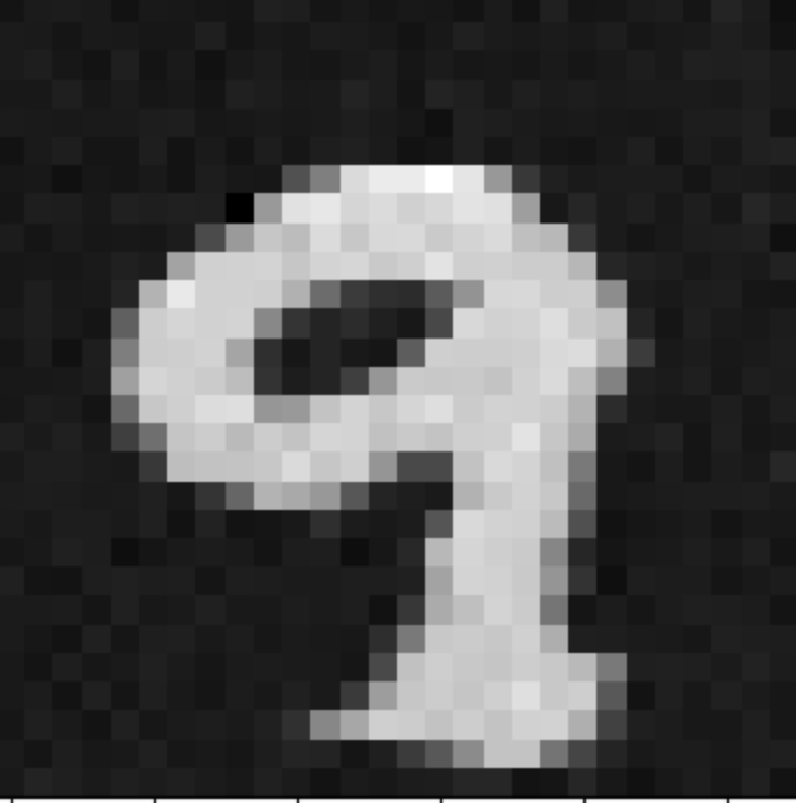
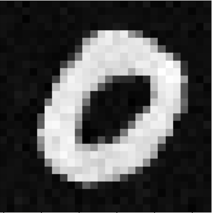
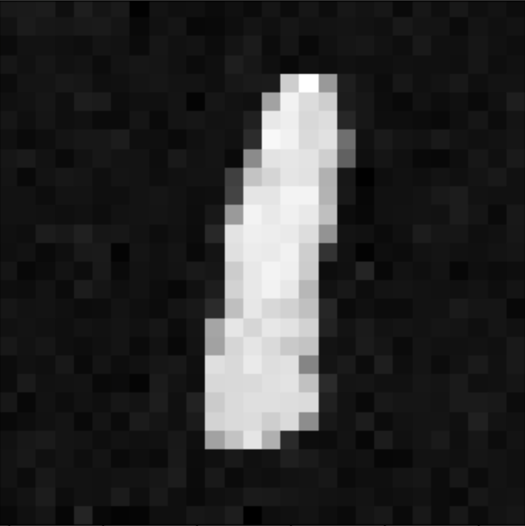
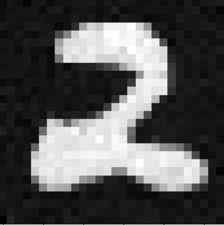
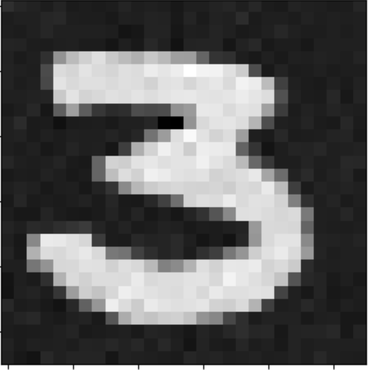
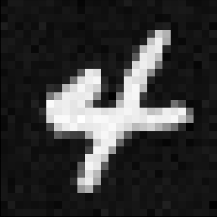
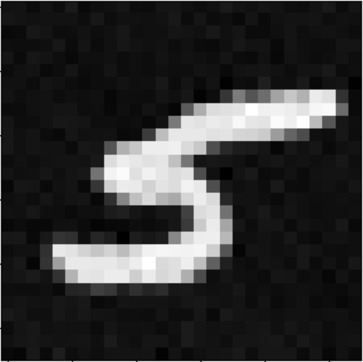
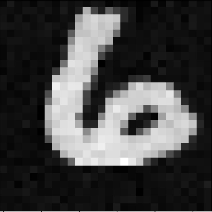
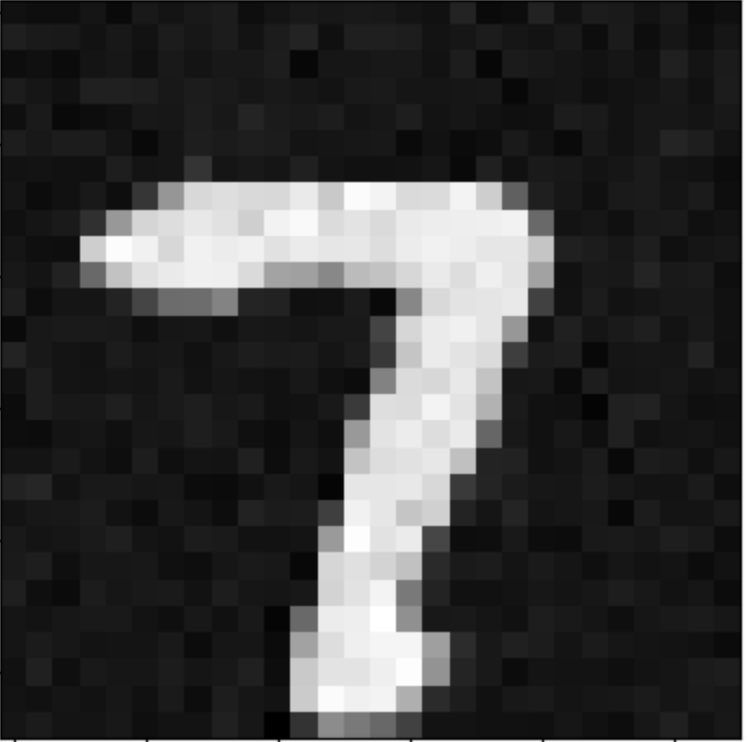
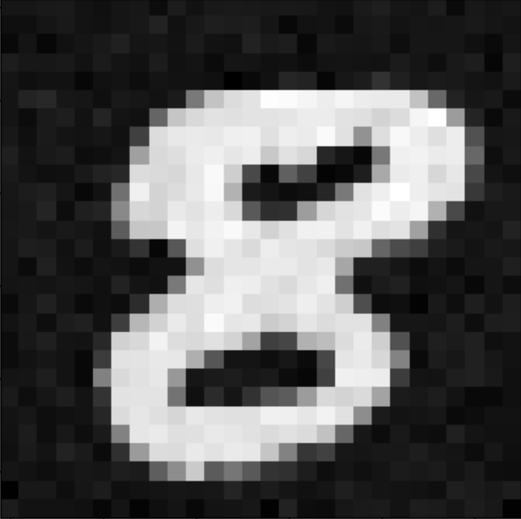
Results of the model shown at 20 epochs is shown below.