Image Rectification & Mosaics
By Ajay Bhargava
Image Warping
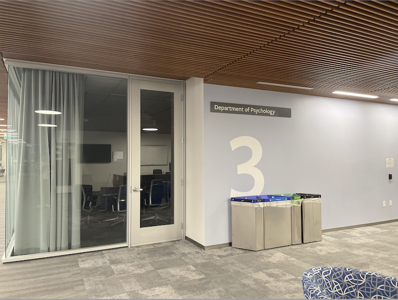
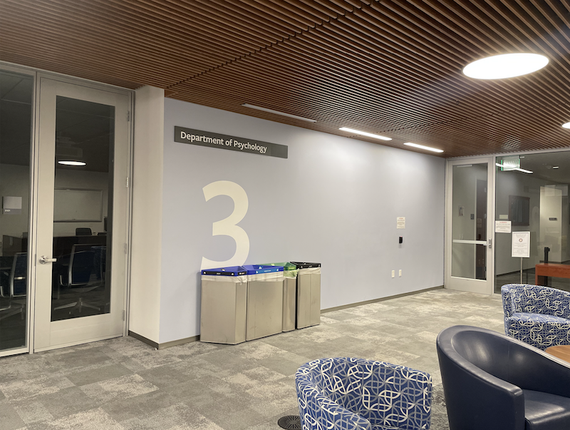
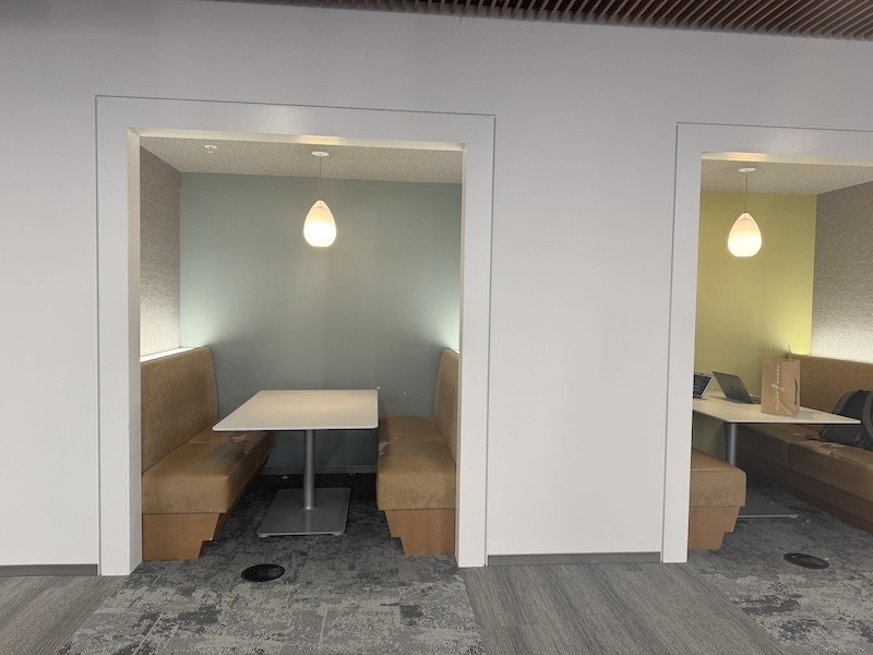
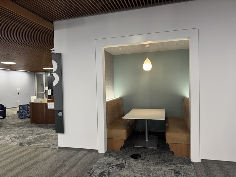
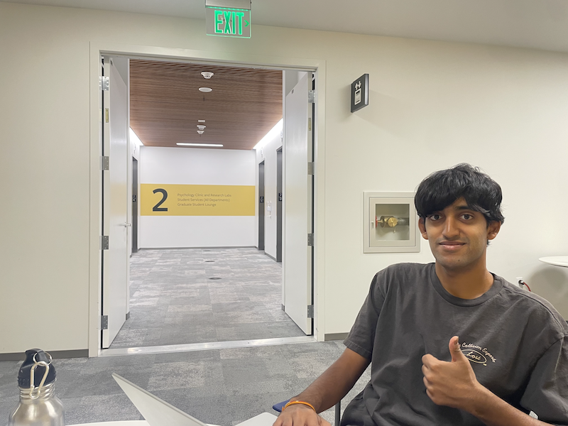
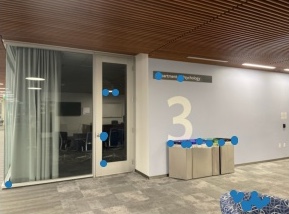
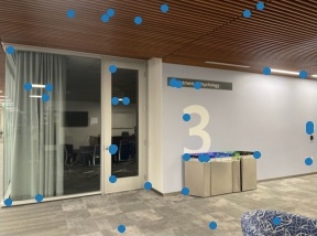
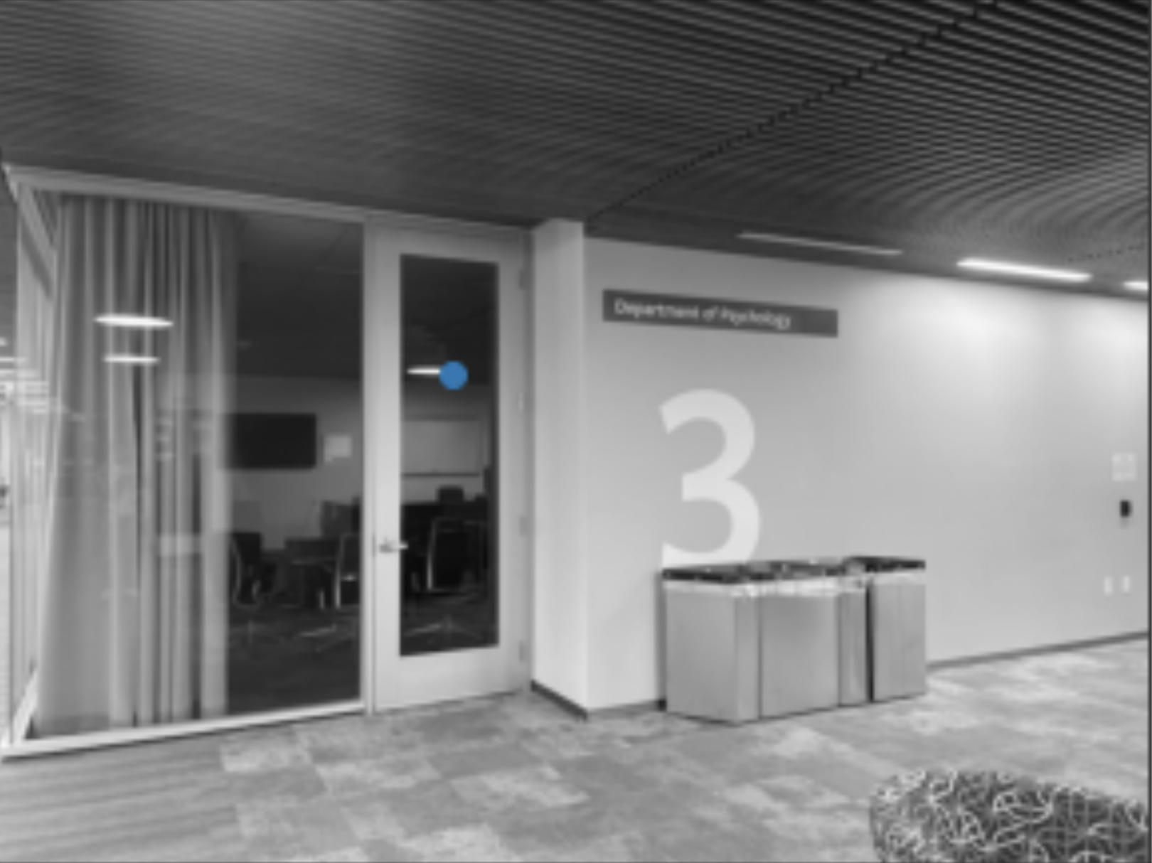
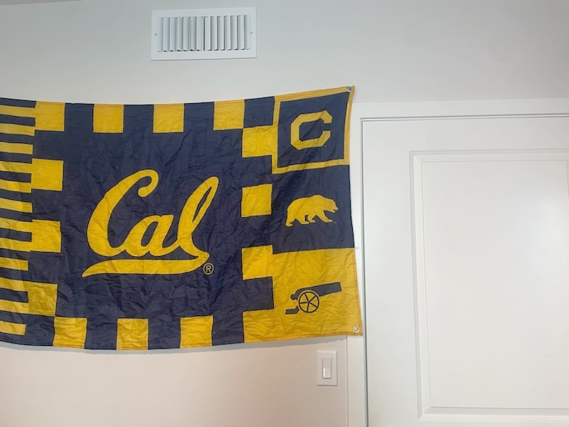
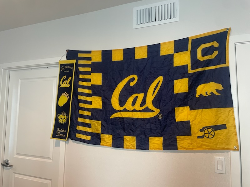
I began this project by shooting sets of images, taken with the same center of projection, but with different angles. These sets of images are shown in this section, as well as the Image Mosaics section, next to their outputs.
To begin warping one image into the perspective of another, I first compute the homography matrix between the two. This gives us a matrix where, when multiplied by a point in one image, it gives us the corresponding point in the other image. Next, I applied this H matrix on all points in one of the images to output it in the perspective of the second image.
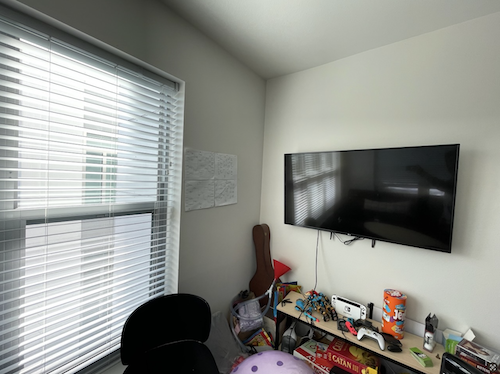
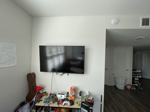
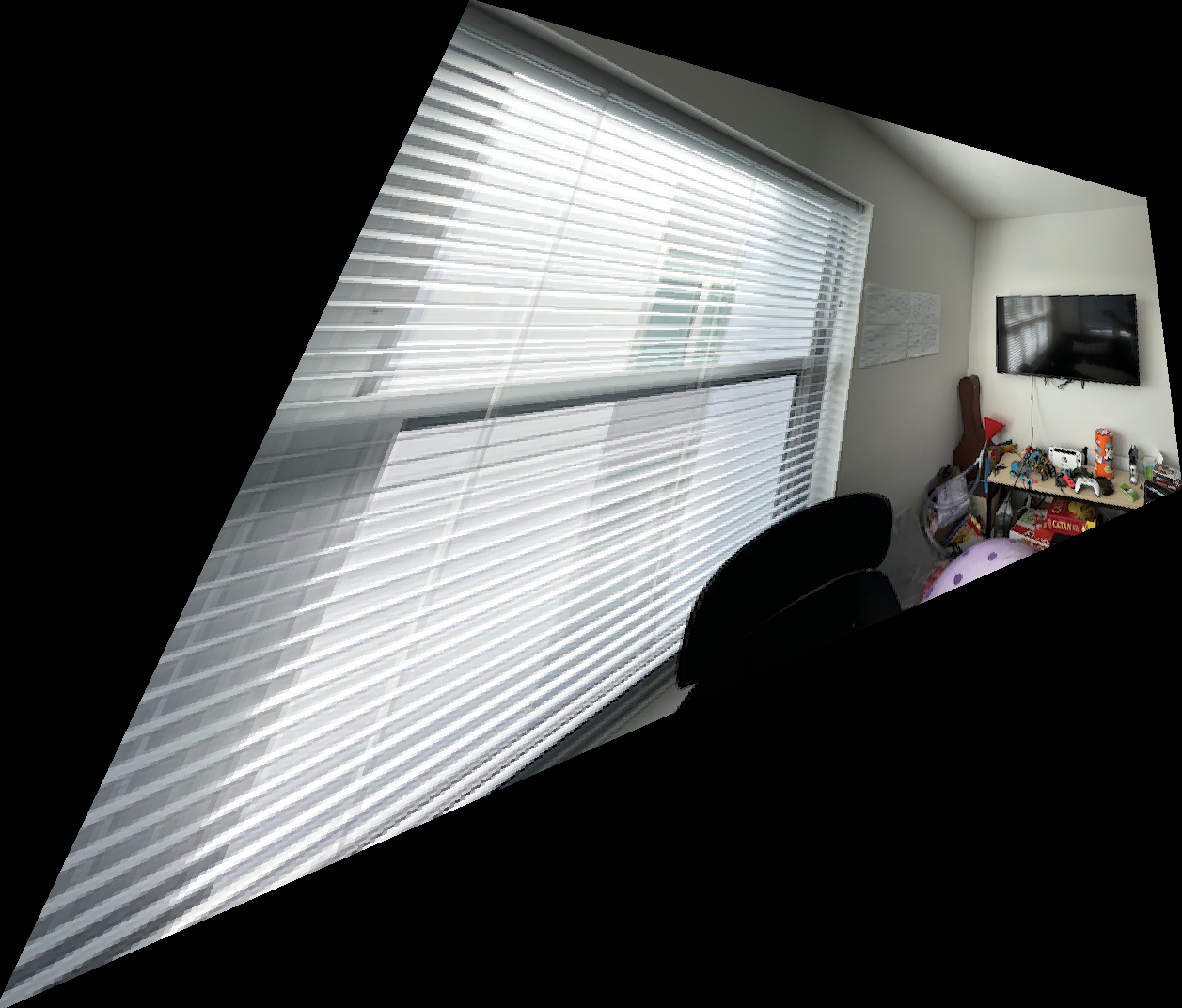
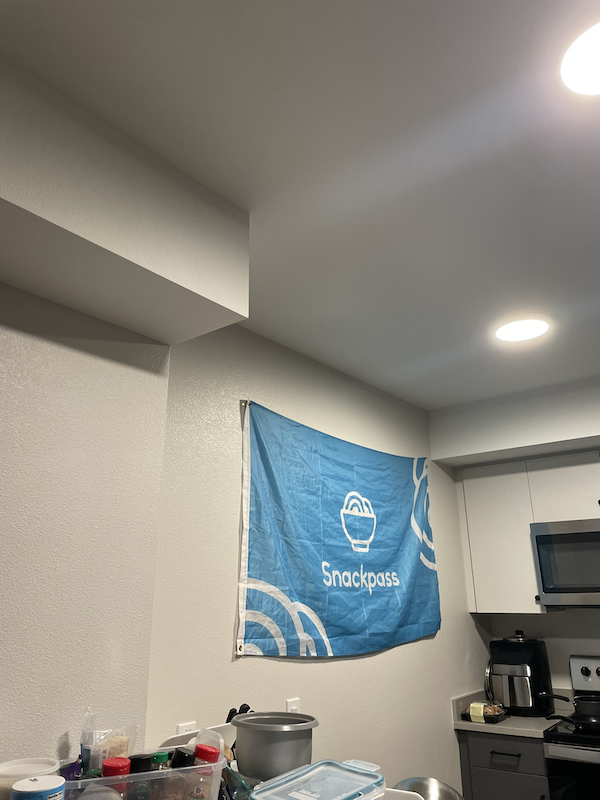
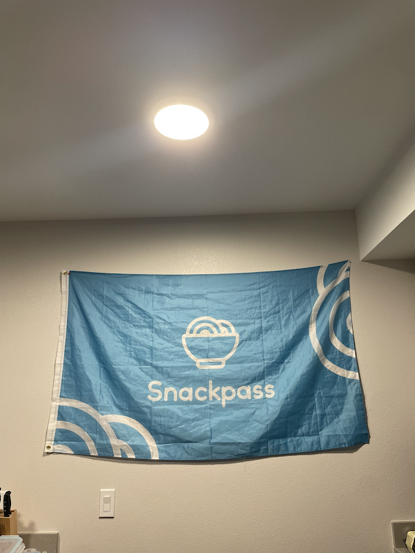
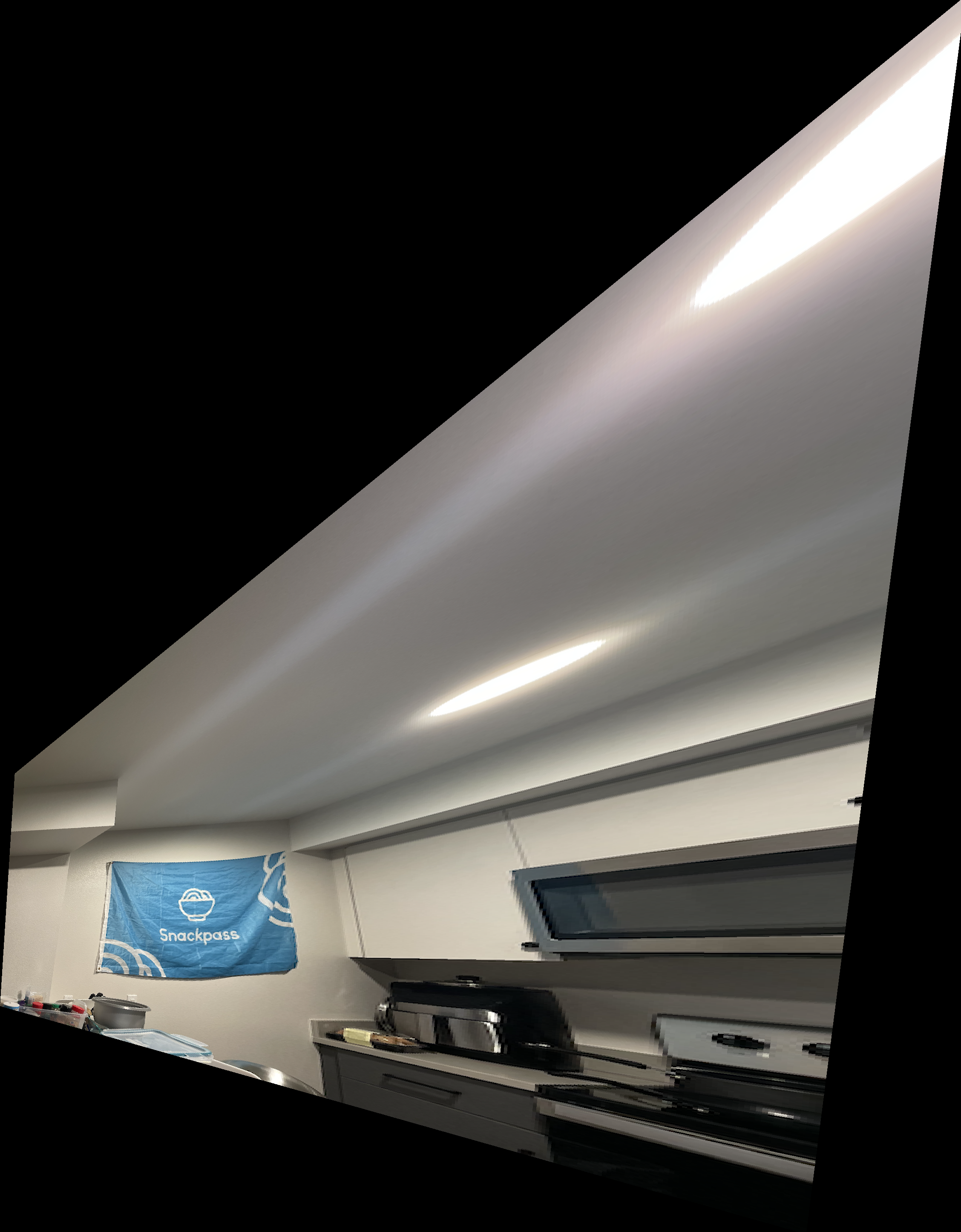
Image Rectification
This similar process can be applied to 'rectify' an image. Some examples are below.
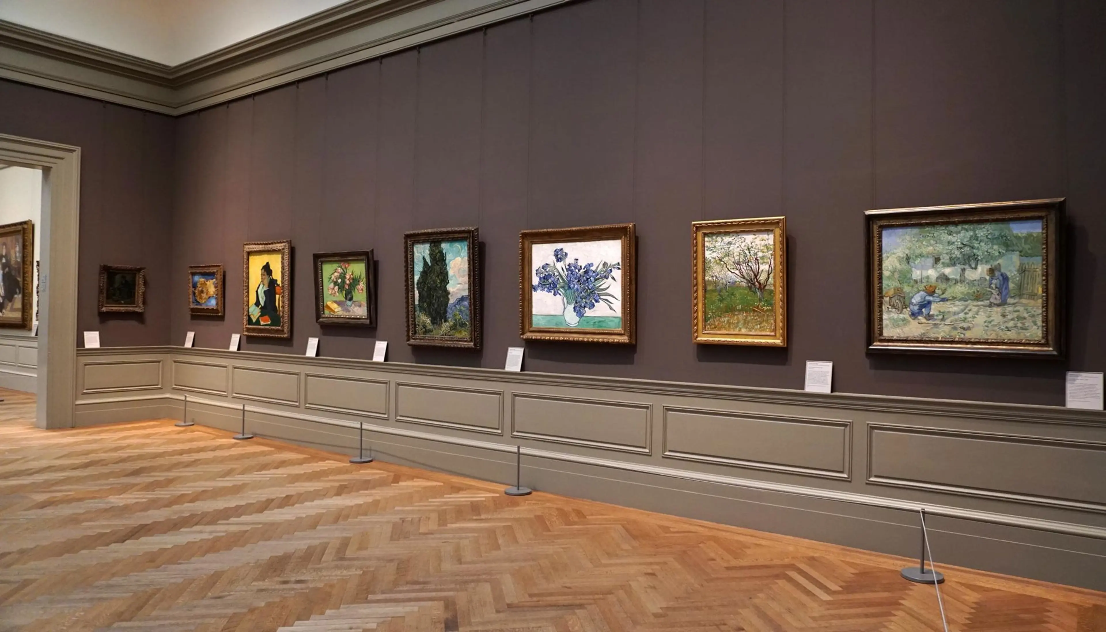
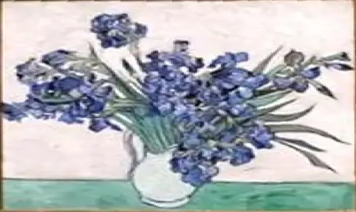

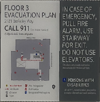
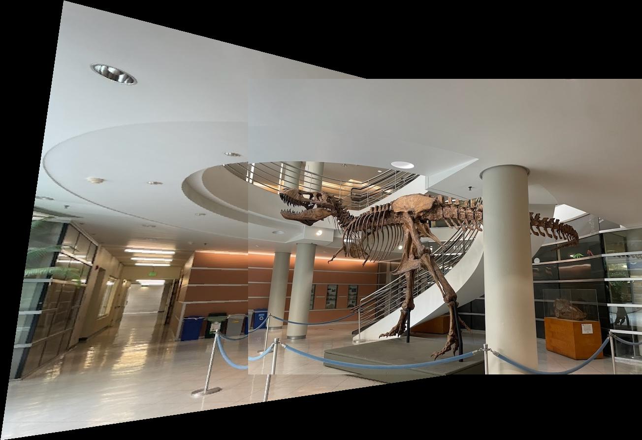
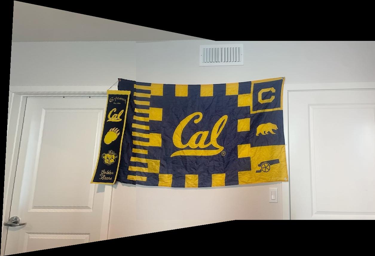
Image Mosaics
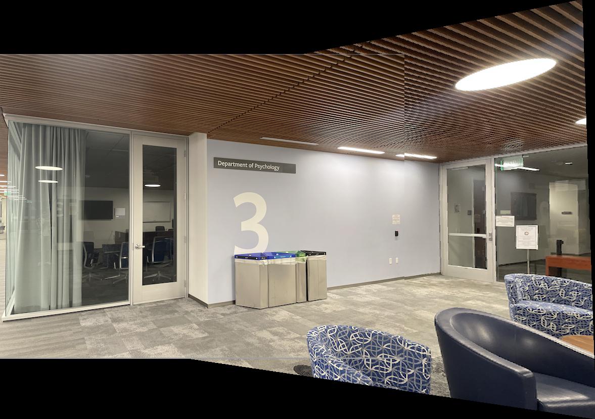
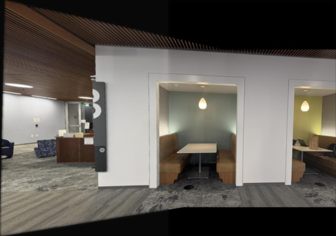
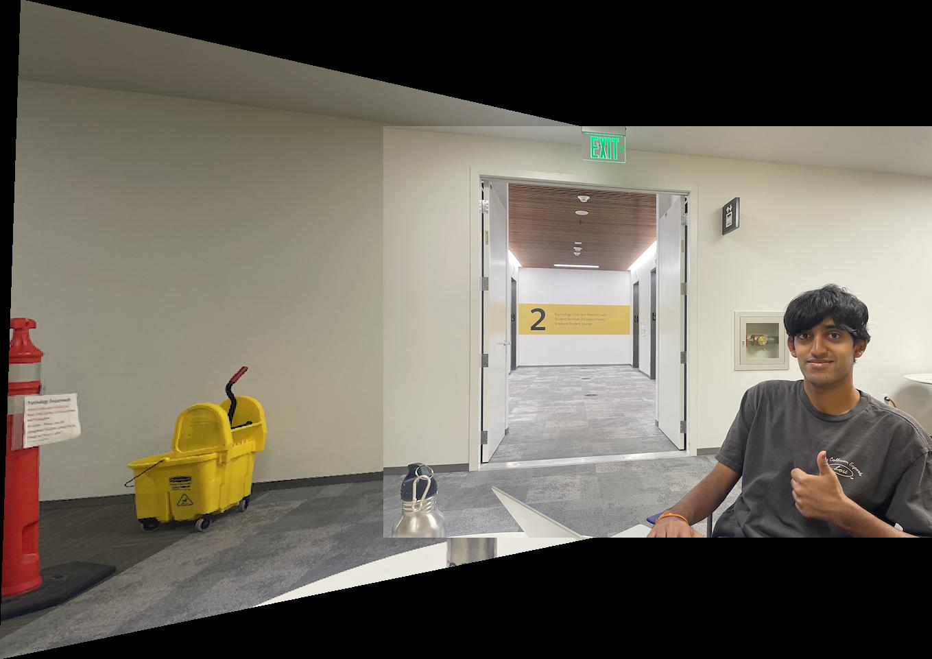
This technique can also be used to create a 'mosaic'. Simply warp one image into the perspective of another, then align them and display. Examples of this are demonstrated below. The slight differences in color are mitigated using a Laplacian Stack, which I implemented at the link here.
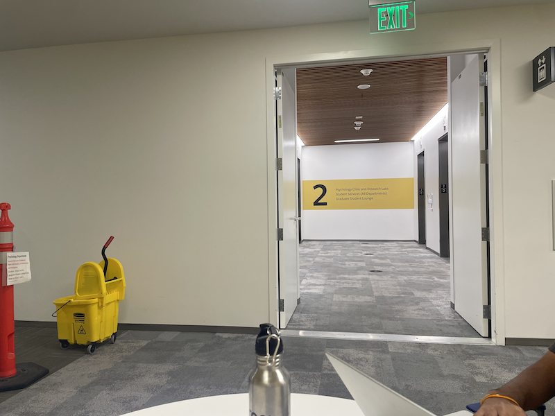
The following is an example of a failed mosaic. First, it doesn't use Laplacian smoothing, so the borders look choppy and are not smooth. The bigest issue however, was not keeping the center of projection this same. This meant objects would not perfectly align, which is clear through the water bottle which was very close to the lens of the camera.
Automatic Feature Detection
The creation of mosaics as shown above requires manual point annotations. The rest of this page will desrcibe a procedure to automatically detect similar features on both images and create the mosaic accordingly. It is based on the paper “Multi-Image Matching using Multi-Scale Oriented Patches” by Brown et al.
The first step in doing so is detecting Harris interest points. The image below demonstrates all of the interest points plotted on one of the mosaic images.
That's way too many points. We can set a threshold to filter out only the most prominent of these points.
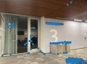
Adaptive Non-Maximal Suppression
The points selected, in many cases, are very similar points that are closer together. To properly estimate the homography, it is desirable to have points spread out across the image, though still remaining important Harris points. I implemented the Adaptive Non-Maximal Suppression technique from Brown et al. An example result of the ANMS technique is shown below.
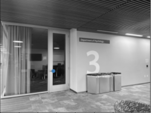
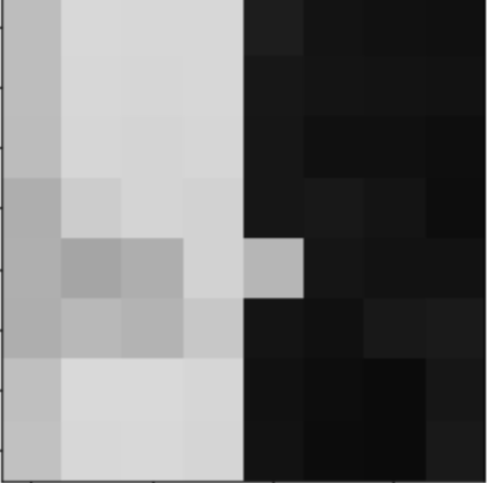
Feature Descriptors
In order to find ways to match the points from one image to another, I implemented feature descriptors accoring to Brown et al. A 40x40 window around each point was taken, blurred, then sampled down to be 8x8. This array can then be flattened and compared to the descriptors from the points in the other images. Examples of a point and its corresponding descriptor (before flattening) are shown below.
Feature Matching, RANSAC, and Mosaics
I compared the feature descriptors for each point to the descriptors of the points from the other image. Using the algorithm described in the Brown et al. paper, we compare the 1-Nearest Neighbor with the 2-Nearest Neighbor, and if the ratio of these is below a set threshold, then we include this as a match.
From here, I performed a random sample consensus (RANSAC). The idea is essentially taking 4 random points at a time, and determining the homography based on these 4 points. The number of outliers and inliers are counted for each homography, and we simply choose the one with the largest number of inliers as our homography matrix. We use the list of inliers as our input points for the exact procedure as described at the beginning of this page/project.
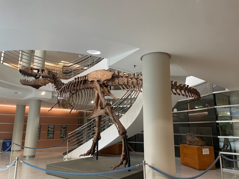
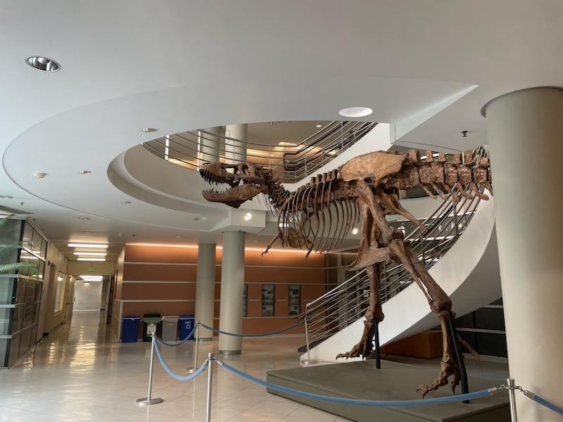
The following are examples of mosaics made from the automatic feature detection method, the first is the same input images as part 1, the rest are new mosaics.

Takeaways
The most interseting takeaway from this project for me was the RANSAC algorithm. It was unique to see a randomized algorithm put to use, as though I have studied things like this in the past before, I have never truly used in a project before. It is interesting how these mosaics are non-deterministic due to the fact that the algorithm is randomized, yet the reslts will be extremely similar despite the randomness.