Filters and Frequencies

Filters

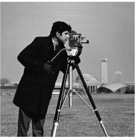
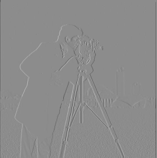
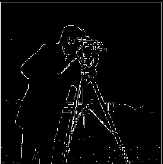
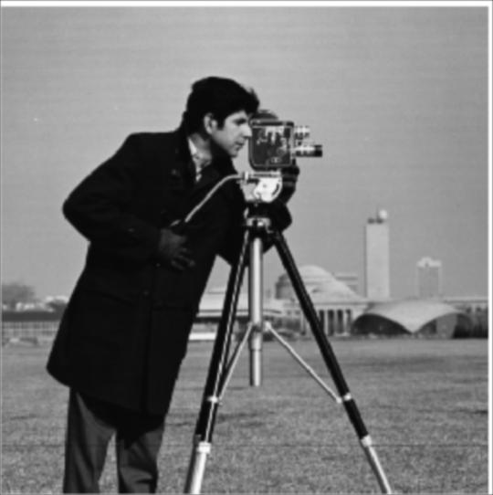
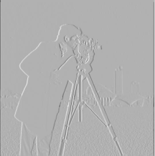
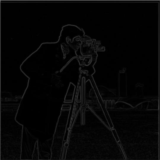
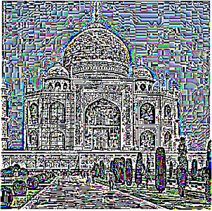
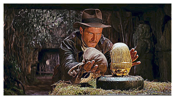
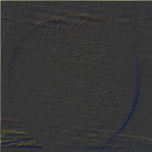
This section demonstrates edge detection using filters. The first set of images below demonstrate a basic finite filter using the difference operators [1 - 1] and its transpose. Combining these values by taking the root of the sum of squared pixel values yields the gradient image. This image was then binarized using a threshold of 0.25, yielding the final edge-detected image below.

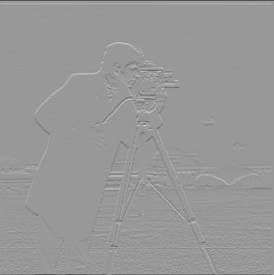
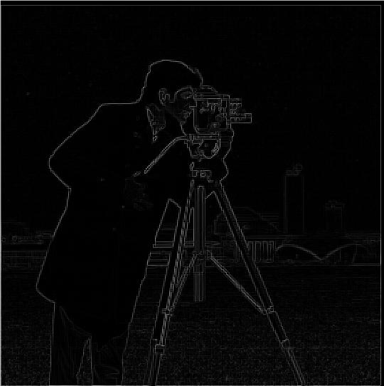
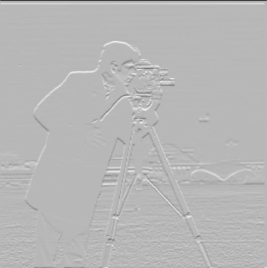
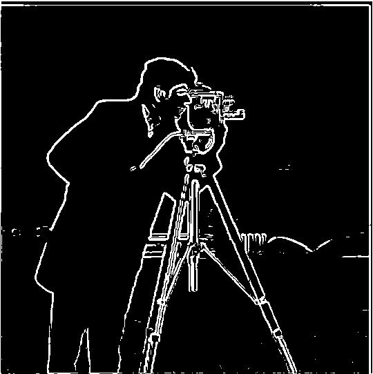
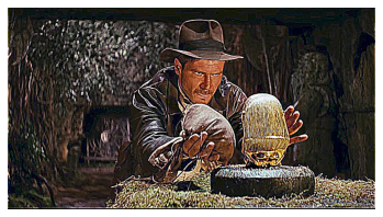
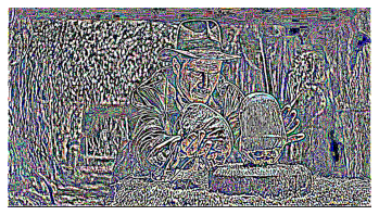
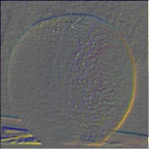
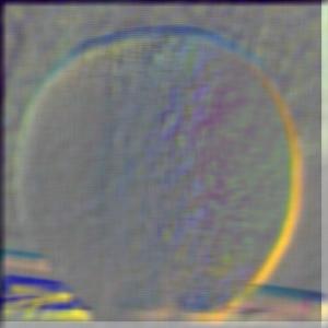
In order to improve the edge detection quality, a derivative of gaussian filter was used. The image was blurred using the Gaussian filter prior to running the finite difference filters on it, diminishing the amount of noise in the final output. A threshold value of 0.09 was used to binarize the image. This yielded the output below.

As a method to authenticate the result, a single filter was created by convolving the Gaussian filter with the finite difference filters. The image convolved with this filter would be expected to yield the same results as the method above – and it did.

The main difference with using the gaussian filter is the lack of noise in the output result. The edges detected are more defined, and the background of the image has less false detections. Using the blurred image as the input also changed the ideal threshold value to be significantly lower.

Sharpening

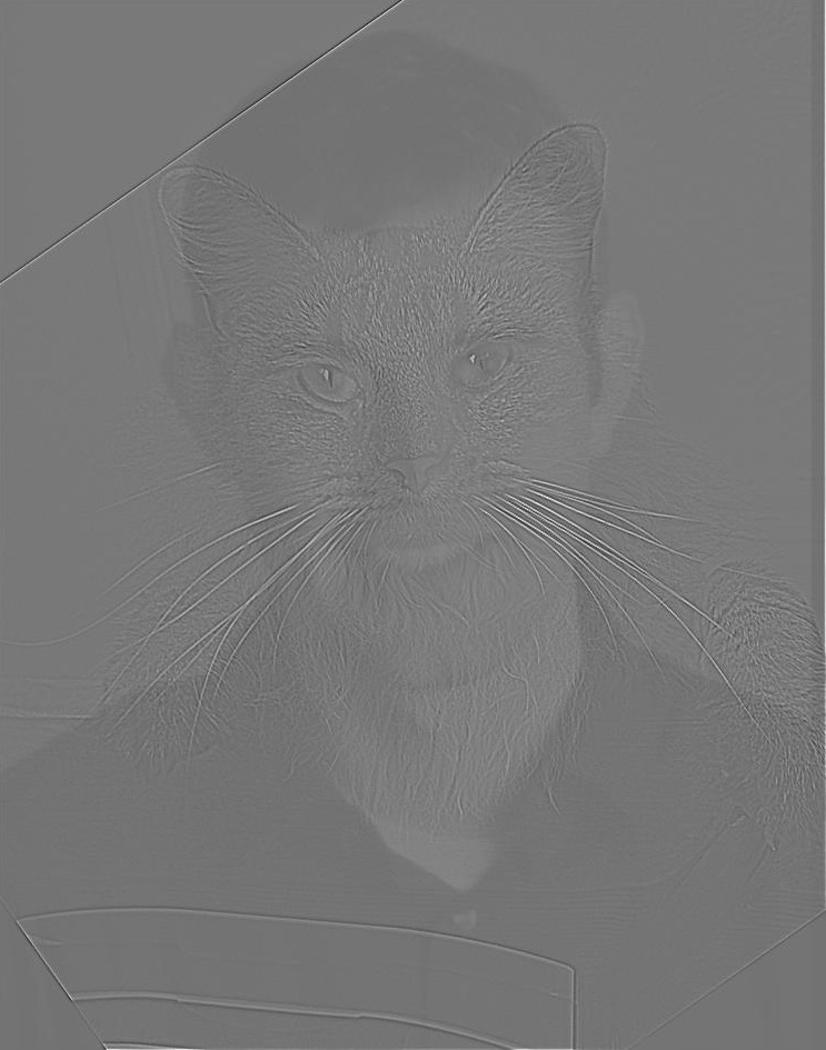
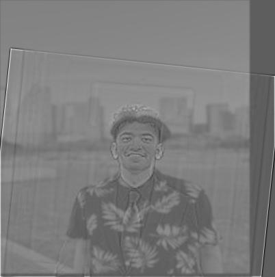
Using a similar Gaussian filter as described in the sections above, I extracted the low and high frequencies of an image in order to perform sharpening. By adding the high frequencies of the image, multiplied by some value alpha, to the original, it achieves a sharpening effect. This is demonstrated on two sample images below.

A similar process was followed in order to blur an image, and then attemp to resharpen it to its original. The image was blurred with a Gaussian filter, then this resulting image had its high frequencies added to itself. The reconstructed image is displayed below.

Hybrid Images

Using the extracted high and low frequencies as described above, I create 'hybrid images'. These are images that when looked at from a distance shows a different image than when looked at closely. This is due to the fact that the high frequencies are more visible from a shorter distance, while the lower frequencies are more visible from a further distance.

+

=

+

=

+

=

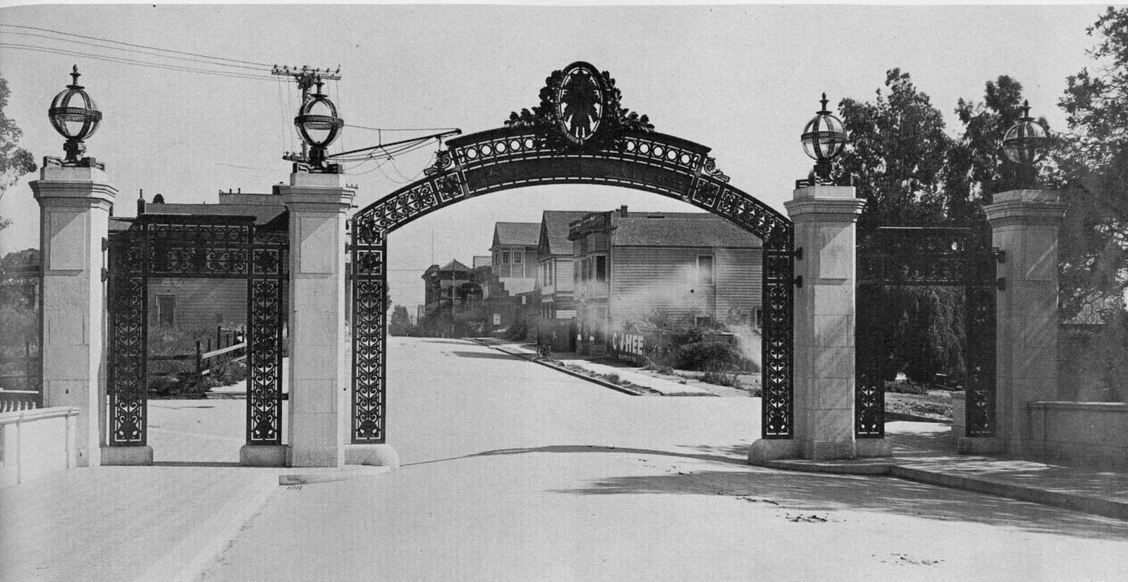
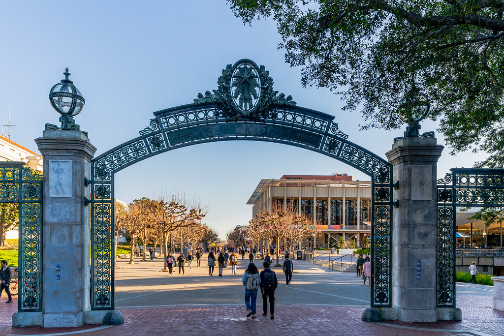
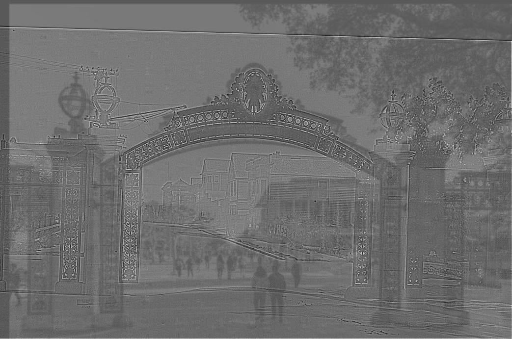
The first two hybrid images appear to work better than the final one. I would suppose this is due to the fact that all of the landmarks of the gate are not perfectly aligned, which causes some issues when perceiving the image. It may not work with trying to layer the same image on top of itself (i.e. the gate is essentially the same in both images, just with different backgrounds).

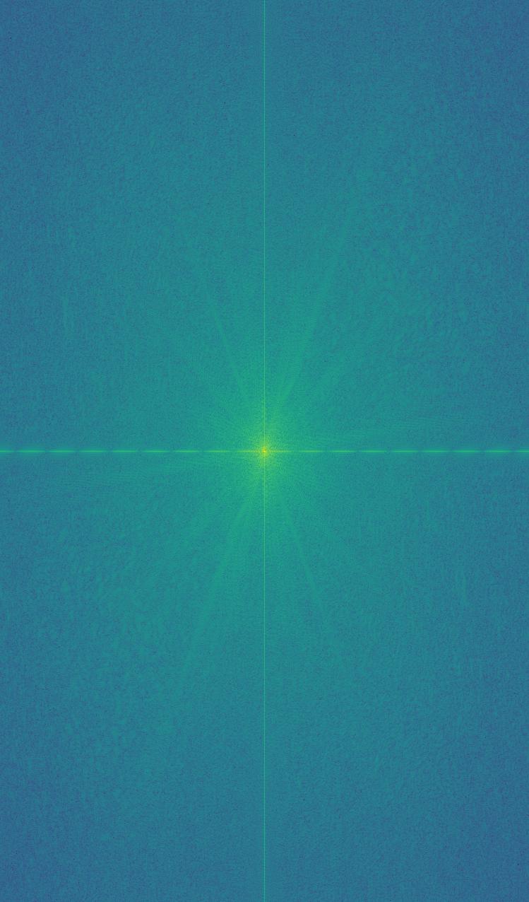
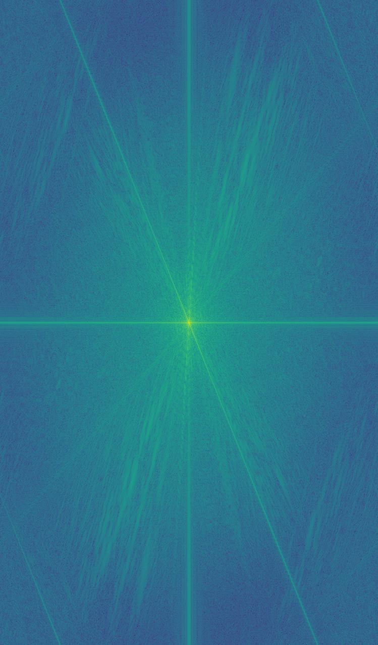
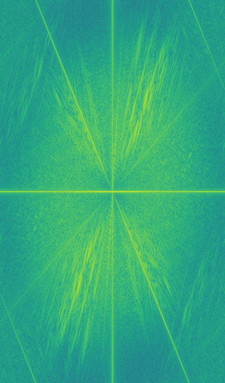
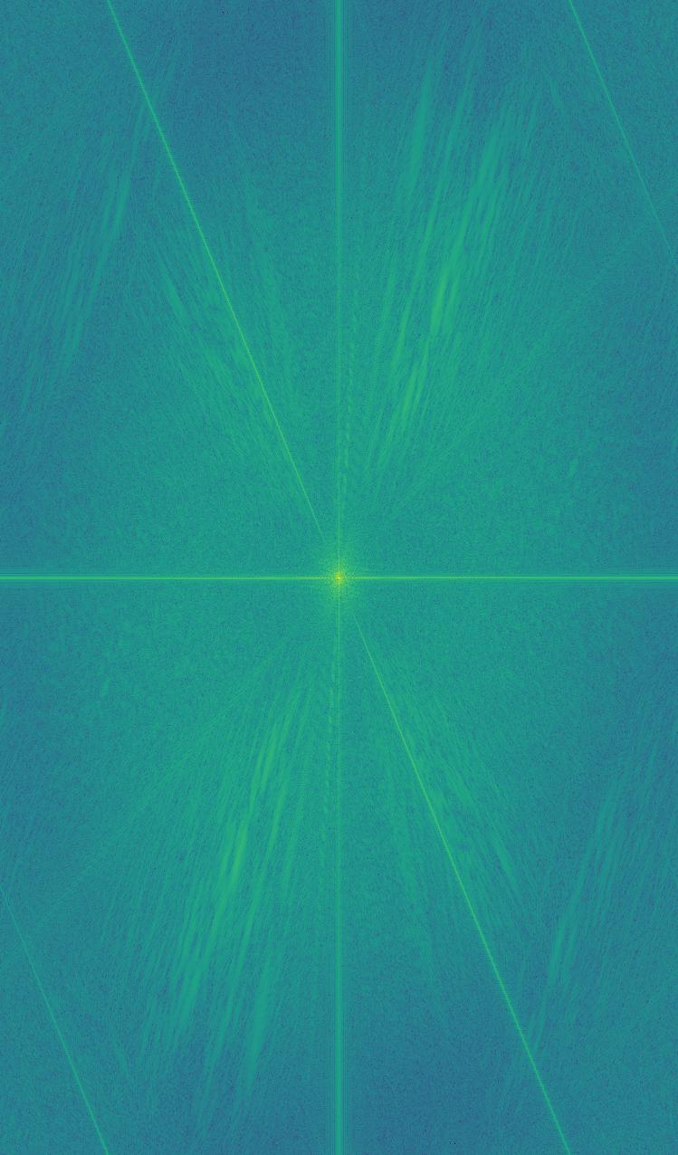
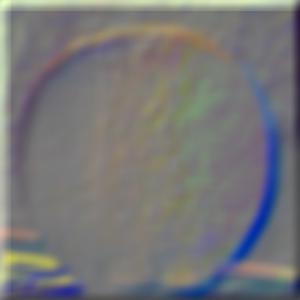
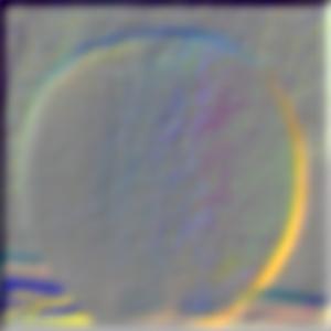
We can also view this process in the lens of frequency analysis. For the Derek & Nutmeg example, the Fourier transforms of the original images, the filtered images, and the hybrid image are shown below.

Multiresolution Blending Through Gaussian & Laplacian Stacks

The following section focuses on combining images using a Gaussian and Lapalcaian stack. A Gaussian stack is a series of the same image, continuously blurred at increasing levels with a Gaussian filter. A Laplacian stack is the differences between the images in the Gaussian stack, appended with the final image in the Gaussian stack at the end. Summing up the images in a Laplacian stack yields the original image at the beginning.

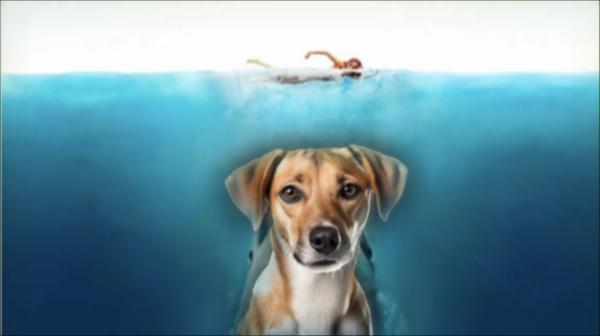
This technique can be used to combine images in a smooth manner. By combining the Laplacian stacks of two images along with the Gaussian stack of a black and white mask, the images can be summed up to create a smooth blend, as demonstrated below.

+

+

=

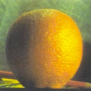
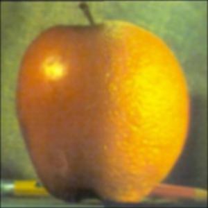
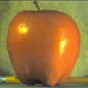
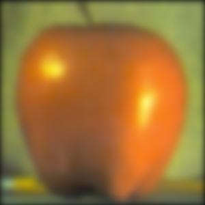
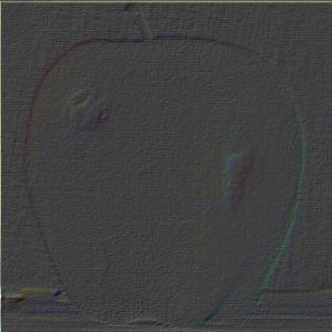
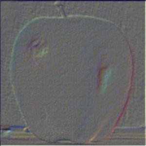
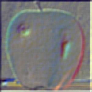
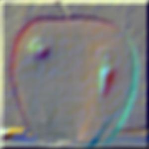
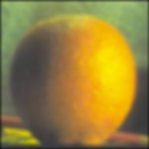
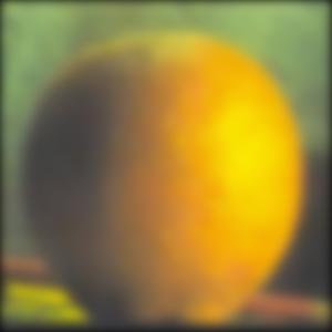
Below are the Gaussian and Laplacian stacks for the apple and orange, respectively. The entire stack is not shown for brevity.

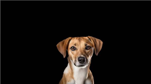
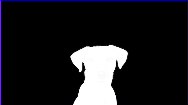
Below are a few more examples of the algorithm at work, with differing masks.

+

+

=

+

+

=

Takeaways

Attempting this project allowed me to better understand filters in regards to computational photography. Specifically, the point I found most interesting was the simplicity in creating images such as hybrid images, or sharpening an image. It is simply a convolution and can be combined into very few steps, which was demonstrated above. When I edit my own images by sharpening them, I'll now understand how it's done.